The default setting is to have the grouping icon below the grouped rows. But you can switch things and have the icon at the top of the grouped rows.
Category Archives: Data
Creating Groups for Power Queries in Excel
Put some order in your queries
Once you start to use Power Query you may find yourself with quite a few queries in the one file. To make it easier to control them you can use groups to keep similar queries together.
Excel Sort within a Sort
Colour by numbers
Did you know you can sort by colour in Excel? Did you know you can sort ascending or descending within that colour? I was asked a question in a recent webinar and in answering I found out that you can sort within a sort.
Free Webinar Recording – Excel Chart Tips and Tricks
Feedback score 94.5% based on 59 responses
In November 2019 I re-ran my Excel Chart Tip sand Tricks session.
The detailed pdf manual and example file can be downloaded using the button below. Content listed below the video.
CPD note – if you are claiming CPD for watching this recording you need to keep your own records. People who attend the live sessions receive an annual listing of attendances.
This webinar is focused on showing you how to create and modify charts in Excel 2016 with a minimum of fuss.
The Chart interface changed in Excel 2013 and I take you through some of the changes.
You will see best practice design and formatting techniques demonstrated and explained.
See how to create dynamic charts that automatically change based on selections made or data added.
Learn about the feature added in Excel 2010 called Sparkline charts.
I also include some useful date-based functions.
Extracting initials in Excel
Handling a space or a comma separator
If you have a system that uses initials to identify people then being able to extract initials from a first name and last name combination can be handy. A formula can automate the process and there is also a quick, manual way to do it.
Top 5 reports with PivotTable and PivotCharts
Switch the order of the Axis
When you create a top 5 sorted report with a PivotTable, the Pivot Chart isn’t always what you expect, there is an easy solution.
Changing the Close & Load settings in a Power Query
Its a right click option
A recent attendee at a webinar posed the question, can you change the Close & Load setting on an existing query? Here is the answer.
Free Webinar Recording – Excel Formula and Function Tips
Feedback score 95.8% based on 66 responses
In October 2019 I re-ran my Excel Formula and Function Tips session.
The detailed pdf manual and example file can be downloaded by using the button below. Content listed below the video.
CPD note – if you are claiming CPD for watching this recording you need to keep your own records. People who attend the live sessions receive an annual listing of attendances.
This session covers lots of tips, tricks and techniques to speed up the formula creation process. You will learn:
- how to quickly start a formula
- the benefits of the numeric keypad
- to use AutoComplete to save typing
- how to easily insert $ signs to fix references
- about the calculation sequence
- how to use the colours Excel displays when editing formulas
- the tricks on selecting large ranges
- using formulas and Format as Table together
- a helpful technique when working with ranges in other sheets
Free Webinar Recording – Introduction to Power Query
Feedback score 94.5% based on 91 responses
In October 2019 I ran my Introduction to Power Query webinar for free (previously it was a paid session). I want to get this information out to as many people as possible. please share this resource with colleagues and your network.
The detailed pdf manual and example file can be downloaded by using the button below. Content listed below the video.
Power Query allows you to automatically perform data cleansing routines on your data sources – no manual intervention required. Simply refresh and your data is ready to use. You can use csv files; txt files; databases and existing Excel tables as your data sources. Learn the basics, plus an advanced technique to automate data cleansing routines on your data sources.
CPD note – if you are claiming CPD for watching this recording you need to keep your own records. People who attend the live sessions receive an annual listing of attendances.
This session covers
- fixing dates so that Excel can recognise them
- formatting columns as text – retaining leading zeroes in CSV files
- deleting unwanted rows and columns from your data
- removing leading and trailing spaces
- populating blank values with zeroes
- populating blanks with entries from above
- correcting trailing minus signs
- unpivot a report – how to convert a report layout into a data table layout
- converting a MYOB report into a data table
Hiding Zero Rows in Excel with No Macros
Filter technique
Over the years I have had regular requests for a technique to hide zero rows in reports. You can use macros but you can also use filters. Let’s see how you can implement a filter solution.
Restricting column inputs based on the current month
A data validation solution
Let’s say you have an input range that covers the whole year. You only want users to make entries in the current month column. How can you limit the month entry? The answer is a custom Data Validation.
Power Query Fill Down Doesn’t Work
The fix is easy
Sometimes when working with CSV files in Power Query you may strike the situation where Fill Down doesn’t fill down. Don’t worry there is an easy fix.
Format as Table Extends Data Validation
Another advantage to formatted tables
Excel’s Format as Table feature on the Home ribbon has many advantages. One advantage that isn’t mentioned much is the automatic extension of Data Validations.
Avoiding keyed in values in Excel formulas
Table solution
One of the cardinal rules of Excel is don’t key-in a value into a formula if that value could change. Tracking the value down could be problematic if you need to change the value. Tables can be the solution to avoiding keyed-in values.
Excel Comments (Notes) and Freeze Panes
Row height solution
Inserting a Comment (renamed to Notes in newer versions of Excel) in the first row and then using Freeze Panes to keep that first row visible can cause issues displaying the Comment (Note). Here’s how to fix it.
Multiple Entries in an Excel Filtered List
Ctrl key to the rescue
When a list is filtered you are only seeing the rows that match the filter. The other rows are still there, just hidden. If you want to make the same entry in a group of filtered cells you can’t use the fill handle to drag and copy as you will overwrite the hidden rows. There is an easy way to do it.
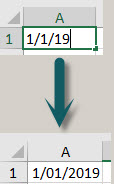
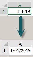
Entering Dates in Excel
Stop the full stop
There are only two characters Excel recognises when separating numeric days, months and years in dates. They are the / and – characters.
Please don’t use the full stop as Excel won’t recognise it as a date.
Below you can see examples of using / and – in dates.
When you use the full stop Excel won’t recognise it as a date – see below.
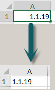
Its left aligned and will be treated a text.
Pasting or inserting with a Formatted Table
When a little icon makes all the difference
When you need to paste new rows to the bottom of a formatted table, or insert blank rows at the bottom, one way is much quicker than others when working with large, complex models.
Unique Entries in Excel via a Conditional Format
Filtering to the rescue
Excel’s Conditional Formatting feature has a built-in unique option. Its unique option only identifies entries that are not repeated. This is different to the Advanced Filter Unique option which lists each unique item from a range once. To filter by entries only appearing once you can use Conditional Formatting with filtering. No formulas required.
Free Excel Webinar Recording – Format As Table Features
Feedback score 93%
In February 2019 I demonstrated how to use the Format as Table feature in Excel, including some advanced techniques.
CPD note – if you are claiming CPD for watching this recording you need to keep your own records. People who attend the live sessions receive an annual listing of attendances.
Many of Excel’s features and functions work seamlessly with formatted tables. They can help you improve the structure and reliability of your spreadsheet files.
Formatted tables can allow you to create powerful reports like those in a relational databases.
Topics covered
- advantages and limitations of formatted tables
- keyboard shortcuts
- using formatted tables with formulas
- solutions to some of the limitations of formatted tables
- using range names with formatted tables
- using formatted tables with data validations
- creating a running total
- using PivotTables
- Relationships (Data tab)
As always there will are a few more tips and tricks shared in the session.
PivotTable Grouping
Create your own categories
Grouping of dates in Excel’s PivotTables is fairly common and in the most recent versions of Excel, automatic. Many people don’t realise that you can perform other types of grouping in Excel.
Improved Data Structure
Tables rule
I ran a webinar in January 2019 where I presented and explained a budget challenge file I had submitted in November 2018. I mentioned during the session that I didn’t like the layout of the Data tab. Well someone asked how should it look? So here is how I would have arranged it.
Free Excel Webinar Recording – Budget Challenge
Feedback score 93%
In January 2019 I presented a webinar that examined a solution to a 4 dimension budget challenge. Download the materials using the button below and watch the video.
CPD note – if you are claiming CPD for watching this recording you need to keep your own records. People who attend the live sessions receive an annual listing of attendances.
NOTE: This is not a beginner’s session.
This webinar is based on a budget scenario which you need to read before the session starts. It is only 3 pages long and included in the materials.
Topics covered include
- using INDEX-MATCH (better alternative to VLOOKUP)
- 3-D formulas and techniques to make using them easy
- using a reporting template
- validations
- extracting sheet names
- automating reports
As always there will are a few more tips and tricks shared in the session.
Extracting entries from a slicer
A simple hack
There is a complicated way to extract the entries from a slicer but there is also an easy way to do it.
Sort by value ignoring the sign
An absolutely simple function to the rescue
I recently received an unusual request about sorting. They wanted to sort in ascending order but they wanted to ignore the sign of the values. So -44 would be next to 44.
Open the Filter Drop Down
If you have filters turned on and you are in the heading row of the table you can press Alt + down arrow to open the filter drop down.

You can then use the arrow keys to move up and down.
Related Posts
Counting Entries in Excel
SUMPRODUCT solution
Excel has a few counting functions. But when it comes to counting entries in a cell it can be difficult if you are using formulas that return a blank cell. This is where the SUMPRODUCT function can come to the rescue.
Distinct Count in Excel
The Data Model to the rescue
Counting is the poor cousin to summing in Excel. Not many people count things, but everyone adds up things. There is a special sort of count that can be useful. A distinct count counts unique entries and is hard to do with a formula. If you have Excel 2013 or a later version you can use a PivotTable to perform a distinct count.
Bold Your Headings
Apparently this is not widely known, but you should always bold the headings in your tables.
Then when you use Format as Table (Ctrl + t) on the Home ribbon tab the header row will be correctly identified.
This also applies to the Ctrl + Shift + L shortcut to insert the filter drop downs.
It also applies to the ranges used for charts.
In general ALWAYS BOLD your headings – it is something Excel looks for.
Ctrl + b is the bold shortcut.
Excel VBA to Remove Filters
Its a one liner
When creating macros that work with filters it is a good idea to remove filters at the beginning of the macro code. Here is how you do that.