Here’s another way to create a Step Chart. This one is quicker. I wrote previously about using a scatter plot and error bars but it required a lot of chart changes. This one hacks a line chart and requires no chart changes.
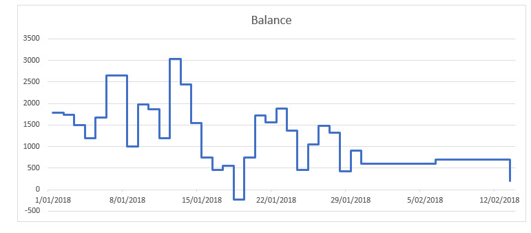
I saw this technique demonstrated here at TrumpExcel and also on Jon Peltier’s brilliant site but it was a manual process. I thought I could automate it. A step chart is shown below.
Excel’s formatted table features allowed me to automate the processes so that as new dates are added to a table the chart automatically updates.
You can download the file with all the formulas using the button on the bottom of this post.
The structure required is shown below. 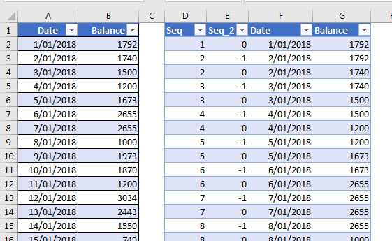
The table on the left is named tblData and holds the dates and values. It needs to be in date sequence.
The table on the right creates the structure we need to hack the line chart to create the step chart.
To hack the line chart all dates require two data points, except the first date.
As you can see all the Balances are duplicated in column G.
The first date is the starting point. After that each date requires two values
- a starting value which is the previous date’s balance
- an end value which is the date’s balance
The formatted table on the right has formulas in all columns. You need to make it long enough to handle the number of dates in the data table. It is completely automated.
The columns and formulas are explained below. Some of them are complex so it might take few reads to understand them. You can use the download file (bottom of post) to easily create your own step chart without out having to worry about the formulas.
Seq column (column D)
This column holds the sequence number to extract the date from the Date column in the table on the left. The value 1 is in the list once, after that all numbers are repeated twice.
The formula is
=MIN(COUNTA(tblData[Date]),ROUND((ROW(D1)+1)/2,0))
Let’s break it down to understand its components.
The MIN function returns the lowest value of two separate formulas.
COUNTA(tblData[Date])
This formula counts how many dates there are in the Date column of the left table. This will be the maximum value displayed in the Seq column because we have used the MIN function around it. Hence the end of the Seq column will repeat the number of dates listed in the left table.
ROUND((ROW(D1)+1)/2,0)
This formula uses a ROW function based on the row above to create the sequence required. By adding one to the row number above and dividing by two within the ROUND function rounding to zero decimal points the correct sequence is created.
The Date column (column F) uses this column (column D) to extract the correct date.
Seq_2 column (column E)
This column is used to adjust the number in the Seq column to enable the Balance column (column G) to get both the opening and closing balances for each date. In the Seq_2 column the first date listed needs to return zero as it is only listed once. Each subsequent date needs an opening balance (previous row) and the final balance (current row).
For all the duplicated values the first value in Seq needs to be -1 in the Seq_2 column to adjust it to refer to the previous row.
The second duplicated number needs to have a zero in Seq_2 as no adjustment is required.
The formula is
=MOD(ROW(E1),2)-1
This MOD function returns the remainder after dividing by 2. Because the formula starts in row 2 and the first number needs to be a zero, I have deducted 1 to get the right result.
Date column (column F)
The column uses the values in the Seq column to extract to the correct dates from the left table.
The formula is
=INDEX(tblData[Date],[@Seq])
This extracts dates from column A based on the number in the Seq column. Because numbers are duplicated in Seq the Dates are duplicated in column F.
Balance column (column G)
This column duplicates all the balances from the table on the left.
The column adds the values in the Seq and Seq_2 columns to get the correct row to extract. The first date returns the first value after that the first duplicated date gets the opening balance and second duplicated date gets the ending date for each date from the left table.
The formula is
=INDEX(tblData[Balance],[@Seq]+[@[Seq_2]])
This extracts balances from column B based on adding the values in Seq and Seq_2. The combinations in Seq + Seq_2 cause the Balances to be duplicated.
Creating the Step Chart
Once you have the correct table structure, creating the Step Chart is simple and quick.
- Select the Date and Balance columns in the table on the right.
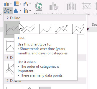
- Click the Insert ribbon tab and select the Line chart drop down and choose the first line charts listed. Click OK.

- Job done.
Adding dates to the bottom of the left table automatically updates the chart.
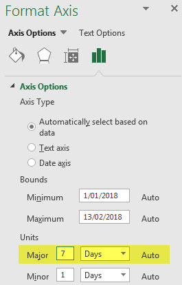
You may want to adjust the date Axis to show weekly dates.
The final chart is shown below.
Hi, I usually designed my own ways around when creating step charts (rather similar to what you show here); you reference Jon Peltier’s site on the subject.
Possibly more recently he added a rather straightforward but more abstract way to achieve this. That works especially well in Line Chart type and with dates, then there is no need to rearrange the dataset into a new set; pls see:
https://peltiertech.com/step-charts-in-excel/ and jump to:
Advanced Step Charts in Excel Line Charts
With the data from your example the formula is:
=SERIES(‘Step Up’!$B$1,(‘Step Up’!$A$3:$A$33,’Step Up’!$A$2:$A$33),(‘Step Up’!$B$2:$B$32,’Step Up’!$B$2:$B$33),1)
This adjusted Series formula gives you the same step chart as yours without creating a new dataset.
Hi Gert – thanks for sharing.