I wanted to offer a solution to a common problem I see in Excel. It relates to creating totals in data that isn’t structured that well.

The list below is a case in point. This is a shortened version of issues that involve 100s of rows.

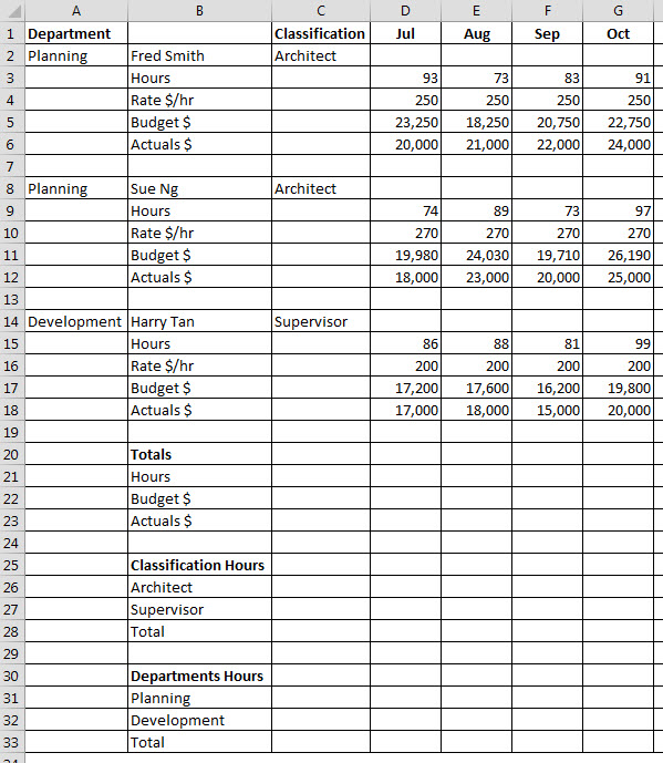
This layout isn’t ideal. I would prefer to change it to a table layout, but we need to work with the existing structure.

We want to populate the totals at the bottom of the page below row 20. Typically the formula used for cell D21 is

=D3+D9+D15

For three cells this is manageable, but imagine if you had 50 employees.

The layout as it stands lends itself to easily summarising the Hours, Budget $ and Actuals $.

We can use a SUMIF to do all the work for us. The beauty with the SUMIF is that if you create the range correctly, it will handle new rows being inserted. That way the totals will automatically update.

Syntax

SUMIF(Range,Criteria,Sum_range)

The formula for cell D21 is

=SUMIF($B$2:$B$20,$B21,D$2:D$18)

The Range is $B$2:$B$20 this contain the entries (Hours, Budget $, Actuals $) we want to summarise. This range is fixed ($ signs added) because we want to copy it across and down.

The Criteria is $B21, in this case we want to add up the Hours. The $ sign in front of B means the reference to B will not change as we copy it across.

The Sum_range is D$2:D$18 this has the values we want to add up. The $ signs in front of the row numbers means they won’t change as the reference is copied down.

Because the ranges have gone as far as row 20, any extra staff added above row 20 will be included.

This formula can be copied to rows 22 and 23 and across to the rest of the year.

The current layout doesn’t make it easy to summarise the hours for the Classifications or Departments.

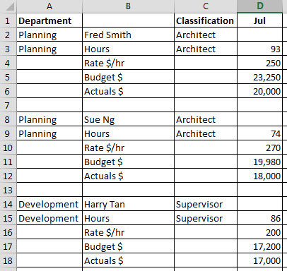
A simple change to the layout can fix this. I have linked cell A3 to A2 and cell C3 to C2. I have copied these formulas down to the Hours rows below – see image below.

The formula for cell D26 is

=SUMIF($C$2:$C$20,$B26,D$2:D$20)

This can be copied across and down one row.

The formula for cell D31 is

=SUMIF($A$2:$A$20,$B31,D$2:D$20)

This can be copied across and down one row.

The final layout is show below.

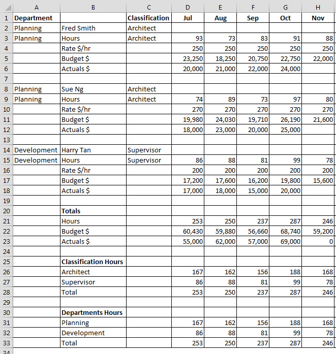
This technique is more flexible and quicker for longer ranges than linking to individual cells.

You can download the file below.

sum_example