Excel’s Conditional Formatting feature has a built-in unique option. Its unique option only identifies entries that are not repeated. This is different to the Advanced Filter Unique option which lists each unique item from a range once. To filter by entries only appearing once you can use Conditional Formatting with filtering. No formulas required.
The data we will use is shown below. 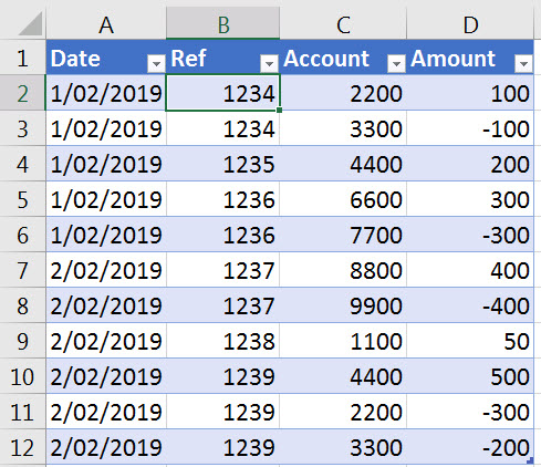
Let’s say it’s a journal listing and every journal number should be repeated at least once. If it isn’t repeated then it is a once-sided journal and that’s a bad thing.
You can download the example file from the button at the bottom of the post.
I have used the Format As Table option (Home ribbon) on this table.
You can read more about this feature at these two links below if you don’t already use formatted tables.
If you want to learn even more about formatted tables I did a webinar in February 2019 covering the topic in detail – see it here.
In a formatted table any column-based formats are automatically extended with the table, including conditional formats.
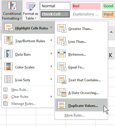
- Select the range B2:B12.
- On the Home ribbon click the Conditional Formatting drop down and choose Highlight Cells Rules, then click Duplicate Values.

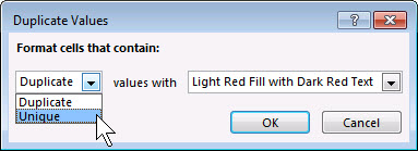
In the left side drop down choose Unique and click OK Unique in this case unique means only appears once.
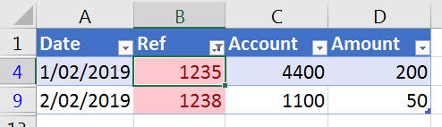
 - The two single entries are highlighted.

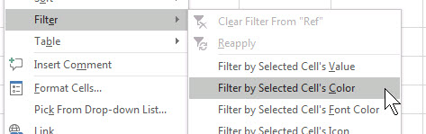
- Right click one on the red cells and choose Filter and then Filter by Selected Cell’s Color.

Job done.
 Unique in this case unique means only appears once.
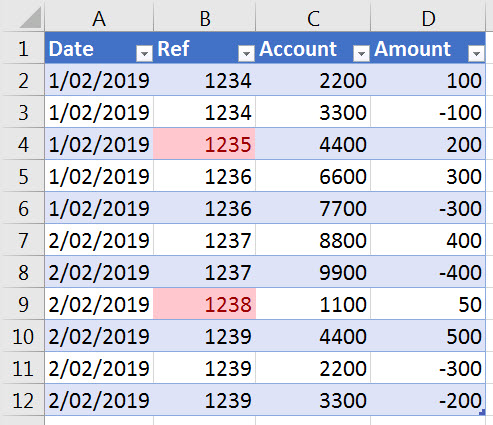
Please note: I reserve the right to delete comments that are offensive or off-topic.