Another post inspired by the book 101 Ready-to-Use Excel Formulas by Michael Alexander and Dick Kusleika. This one is Formula #22 and covers padding entries with zeroes.
Tag Archives: data
Excel PivotTable Subtotal Label Trick
I just learned a new trick for labelling subtotal rows in a PivotTable. Hat tip to Ken Puls MVP of Excel Guru for this tip.
Useful Excel Keyboard Shortcuts for Data Entry
When making entries in Excel there are a few keyboard shortcuts worth knowing. These can save you time and effort.
More Adjusting in Excel
Following on from last week’s post on a single adjustment formula this post will share a more robust solution for including or excluding adjustments.
FILTER Function Technique
An application I use recently updated it’s filtering options to allow you to filter by any filters or all filters. This was a useful addition to the software and I thought that I could apply the same idea to Excel’s FILTER function.
Benford’s Law in Excel – Part Two
Benford’s law is used in auditing to identify data sets that may have been manipulated or adjusted. In my previous post I created a report to analyse a data set based on Benford’s Law. In this post we will create a single formula to create the report and then convert that into a custom function.
Benford’s Law in Excel – Part One
Benford’s law is used in auditing to identify data sets that may have been manipulated or adjusted. In actual data sets when reviewing values the 1st digit of the values tends to follow a predetermined frequency. For example, roughly 30% of the values should start with a 1.
Comparing Averages in Excel
It is common in Excel to use averages to summarise large data sets. It is also common to compare the averages across different segments. Here’s a technique you might find useful when comparing a segment against all other segments.
Excel Power Query Errors List
Sometimes Power Queries generate errors. Some errors stop all data being returned and others will return a blank cell for the error in the returned table. You can list the rows that are generating the errors. This can help you identify what is causing the error.
Excel Power Query and Multiple Files 2023
In this recording of a live webinar I ran in late January 2023 you will learn how to import multiple files in a single Power Query. If you use data at all then Power Query is an essential skill to possess.
Use the buttons below the video to download the materials.
Building on the skills covered in the Introduction session, we will start working with multiple files. For example you may have 12 separate CSV files in a folder. All with the same layout, one for each month of the year. Power Query can import all 12 files as if they were a single file and create a table for the whole year
This session covers
• importing multiple CSV files from a folder
• a technique to capture the file name in a field (column)
• importing multiple Excel files
• merging data from multiple tables
• Extracting header information into a column from multiple CSV files
As always, I shared other tips and tricks along the way.
Introduction to Excel Power Query 2023
In this recording of a live session ran in late January 2023 you will learn how to automate data importation in Excel with Power Query. If you use data at all then Power Query is an essential skill to possess.
Use the buttons below the video to download the materials.
Power Query allows you to automatically perform data cleansing routines on your data sources – no manual intervention required. Simply refresh and your data is ready to use. You can use csv files; txt files; databases and existing Excel tables as your data sources.
Learn the basics, plus an advanced technique to automate data cleansing routines on your data sources.
This session covers
- fixing dates so that Excel can recognise them
- formatting columns as text – retaining leading zeroes in CSV files
- deleting unwanted rows and columns from your data
- removing leading and trailing spaces
- populating blank values with zeroes
- populating blanks with entries from above
- correcting trailing minus signs
- unpivot a report – converting a report layout into a table layout
- converting a MYOB report into a data table
- capture header information in a column
As always, I shared other tips and tricks along the way.
Format As Table Webinar Recording 2023
In this session you will learn all about Excel’s formatted tables. Using Formatted Tables is an essential skill in Excel. Use the buttons below the video to download the materials and completed file.
Many of Excel’s features and functions work seamlessly with formatted tables. They can help you improve the structure and reliability of your spreadsheet files.
Formatted tables can allow you to create powerful reports like those in a relational databases.
Topics covered
- advantages and limitations of formatted tables
- keyboard shortcuts
- using formatted tables with formulas
- solutions to some of the limitations of formatted tables
- using range names with formatted tables
- using formatted tables with data validations
- creating a running total
- using PivotTables
- Relationships (Data tab)
- introduction to dynamic arrays
As always I shared a few other tips.
Selecting a Column Range within a Merged Cell in Excel [video]
I am not a fan of the merged cell format. It causes more problems that it solves. One issue you will face is trying to select a single column range within a range that has a merged cell. Here is how you handle it.
This post is a video post as it easier to show the problem and the solution in a video.
Excel Month on Month Movement
A PivotTable solution
If you need to find the movement from the previous month a PivotTable can be your friend and do most of the work for you.
MIN and MAX and Dates in Excel
Automating the latest date
The MIN and MAX functions can provide easy ways to capture current dates.
Excel Data Validation Blind Spot
Macro to fix it
One of the problems with Excel’s Data Validation is that it is possible to have an invalid entry in a data validation cell. This can be caused by Paste Special Values or linked drop downs that don’t update if an earlier drop down is changed. To easily identify invalid cells you can use a macro.
UNIQUE Function and Blank Cells in Excel
Zero in on a problem
The UNIQUE function has a bit of an issue with blank cells, formulas that return blank cells and zeroes.
Identifying if a List has Unique Entries in Excel
A MODE solution
If you need a logical test to determine if a list is unique you can use the MODE function with the ISNA function.
Data Entry Formats in Excel [Video]
Format as you go
When you enter data into Excel you can format as you type. See how in this short video.
Related Posts
Excel Power Query and Multiple Files 2022
Webinar recording from April 12, 2022
This is the recording of the second free Power Query webinar I ran in 2022.
You can watch the first one at this link.
In this session we see how to import multiple files in one Power Query. We look at importing CSV and Excel files.
You can download the materials, including a detailed pdf manual using the button below.
One Minute to Excel #25 – Find the breakeven point
Goal Seek solution
If we have a simple Profit and Loss and we want to figure out a breakeven point, we can use Goal Seek to find it.
We can also use it to see sales required to meet a certain profit.
All in less than in minute.
One Minute to Excel #24 – 1,000 random dates
A RANDARRAY solution
Let’s say we need to do some testing and we need 1,000 random dates in 2022.
We can use a new function to make this easy to create and easy to change.
RANDARRAY usually works with numbers but in Excel dates are numbers, so we get it to create random dates for us.
I set myself a challenge to do this in less than minute – see how I went in the video below.
Clear the Filter in One Column Only in Excel
Keyboard shortcut
When you have multiple filters across columns you may want to clear just the filter in one column. There is a keyboard technique to do that.
Financial Year Month in a Pivot Table
Create new column
I wrote an article years ago explaining how to use a related table to handle financial years in Excel Pivot Tables. You can read the article here. If you only want the months in financial year order you can just add an extra column to your table.
Handling Multiple Columns in Power Query
Choose Columns drop down
In general, you should reduce the number of columns you import via Power Query to the minimum you require. Here is a quick technique to make that a bit easier.
Show the cells to be removed by Remove Duplicates in Excel
A formula-based Conditional Format
Excel has a Remove Duplicates option in the Data ribbon. It keeps the first item and removes any further items that match.
Excel Power Query and Data Types
Get the Type right
Data types are an important part of Power Query in Excel and Power BI. They define the type of data that should be in a column. When performing some calculations, getting the column data type right is vital.
Conditional Format to Display Only the First Entry
In my previous blog post I showed a technique to reduce clutter. The technique used a manual formatting method. Here is the automated version.
You can see my previous post here.
Below is the original table.
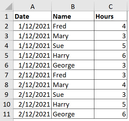
We can use a Conditional Format to only display the first entry of each date in the Date column.
Select the range A2:A11.
Click the Conditional Formatting drop down and select New Rule (third from the bottom).
Select the last option in the top section “Use a formula to …”.
In the formula box enter the following formula.
=COUNTIF($A$2:A2,A2)>1

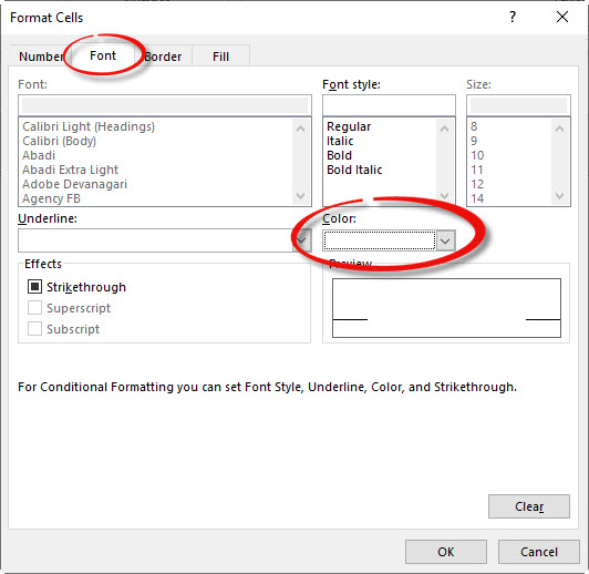
Click the Format button and use the Font tab and change the font colour to White and click OK and then OK again.
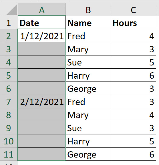
The result is shown below.
The formula for a conditional format must return TRUE to trigger the format. The type of formula that you use is called a logical test, which returns either TRUE or FALSE.
The use of the $ signs is very important in this formula. The COUNTIF function counts the number of entries in a range. If the COUNTIF result is above 1 it is a duplicate. In cell A2 the formula will ALWAYS return 1 as it is counting itself.
When creating a formula-based condition across a range you need to build the formula to refer to the top left cell of the range. In this case we need the range to expand as the range extends down the sheet. Hence, we didn’t use any $ signs on the last two A2 references used.
In cell A3 the formula will be.
=COUNTIF($A$2:A3,A3)>1
This is because the A2 references in the original formula had no $ signs, so they will change with the cell to A3. In our case this COUNTIF will return 2 because the date in cell A3 is a duplicate of the date in A2. This will trigger the format.
This formula expands as the range extends. It uses the cell reference of the cell it is in to determine if the entry is the first entry or a duplicate. This formula will not change the format of the first entry, but it will change the formats of any duplicates.
Input Data Display Hack for Excel
Getting the format white
When creating data input sheets, it is a good idea to use a table layout. Sometimes they can end up looking a little bit busy, especially if you are repeating entries down rows. To help users focus on what they need to do, you can use a little formatting hack to make the layout look a little less cluttered.
One Minute to Excel #23 – Text numbers to real number again
Another solution
One thing you learn quickly about Excel is that there are many ways to achieve the same outcome.
This is another example. In an earlier video I showed two separate ways to convert text numbers into real numbers.
Well, I have just learned another way. An Excel MVP Rick Rothstein shared a third way. I tweaked it and share a keyboard shortcut to do it as well.
Hope you enjoy it.
Added Nov 27, 2021
If you use Text to Columns for other conversion in the same session, you may need to use Alt A E W F as the Delimiter defaults may interfere with the conversion.