If you need to find the highest or lowest three entries in a filtered list you can use the AGGREGATE function to find them.
Category Archives: Excel 2013
Distinct Count in Excel
The Data Model to the rescue
Counting is the poor cousin to summing in Excel. Not many people count things, but everyone adds up things. There is a special sort of count that can be useful. A distinct count counts unique entries and is hard to do with a formula. If you have Excel 2013 or a later version you can use a PivotTable to perform a distinct count.
Auto Format Formulas in Excel
Excel 2013 onwards
Would you like to change the format of all your formula cells so they have a different fill colour or font? There is a way in Excel 2013 onwards.
Copying Without Affecting Relative References
Works for Excel 2013 onwards
There is an easy technique to copy a single formula and paste it without affecting relative references but what if you wanted to paste lots of formulas?
Creating a Unique Dynamic List in Excel
A Power Query technique
There are a couple of techniques to automate a unique list of items in Excel. I have covered them in previous blog posts (see links below). I thought I would describe how to use Power Query to create a dynamic unique list.
Do You Have Excel Inquire?
Its a built-in audit add-in
Inquire is a new add-in in some versions of Excel 2013 and later versions It is an auditing Add-in that can analyse and report on your Excel files.
Export a sheet as a PDF
It takes a few clicks but it is possible
I have previously posted about using CutePDF to create pdfs from Excel sheets. There is another way, but it takes a few clicks and it only works in Excel 2010 and later versions. (It may work in Excel 2007 but I have taken that version off my PC so I can’t test it.)
SUMIFS Function Warning
Leading zeros are not handled correctly
Most people are unaware that the SUMIFS function has a serious limitation when it comes to codes with leading zeroes. This post shows you how to perform calculations involving codes with leading zeroes. This issue also affects SUMIF, COUNTIF and COUNTIFS.
Relationships Shortcut
Excel 2013 added the Data Model to Excel.
The Relationships option (Data ribbon) is part of that model. It allows you to create relationships between tables so that you can use a PivotTable to report on multiple tables.
You have to have used the formatted table option to use Relationships.
See my December 2016 INTHEBLACK article for an example.
The keyboard shortcut to create or edit, a Relationship is easy to remember – it is
Alt a a
Pressed in sequence, not held down.
Show Horizontal Axis Entries Below the Chart
Great for displaying negatives in a line or column chart
I learned about a chart Axis option in Excel during a recent webinar – thanks to one of the attendees. You can show the Axis entries below the chart – this is handy for column charts that display negatives.
Finding the Last Used Cell in an Excel Column
Array free zone
If you need a formula to identify the last used cell in a column you don’t have to use an array formula. The AGGREGATE function can calculate it for you.
PowerPivot and Power Query
How to get and install
I have run two introductory webinars in 2016 on these two topics. You may need to download them and install them before the webinars so you can use them during the webinars. The Add-ins are free from Microsoft.
Day Of The Week
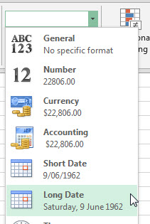
A quick and easy way to find out the day of the week for a specific date is to use the Long Date format from the drop down in the middle of the Home ribbon (in the Number section) – see below.
Flexible Hyperlinks in Excel
Using the HYPERLINK Function
Hyperlinks are a great way to navigate around large spreadsheets. Unfortunately they each take a few clicks to create and can be easily broken. You can use a function to easily create multiple, flexible hyperlinks.
Clearing the tab colour
I use colours on my sheet tabs to signify different things.
To clear a colour, you can use the following keyboard shortcut
Alt h o t n
Pressed in sequence, not held down.
Related Posts
Sequential Numbers With a Twist
How to ignore hidden rows
You want a sequential number in a column. The challenge is, it must display as sequential even if rows are hidden or filtered. Is this possible?
Getting the Week Number From a Date in Excel
New WEEKNUM Function - ISO 8601 standard
Excel has had a week number function for many versions, but Excel 2013 added a new week number function that complies with the ISO 8601 standard week number.
Adding years or months to a date in Excel
Finding the end date can be easy
When working with loans or leases, it is common to have to add a number of years to a start date to determine the end date. An Excel function can automate that process.
Paste Values
After copying, use the following keyboard combination to paste just the values – no formulas or formats.
Alt h v v
These keys are pressed in sequence, not held down.
Working with Imported Dates and Times in Excel
Date data imported from other systems can include times. This can make lookup and other calculations difficult. One function can make removing or extracting time easy.
How to stop overwriting files in Excel
Open a copy instead
Is this you? You open the May file and make the changes for June and save it and then remember you hadn’t renamed the file as June. Well, I’ve done that too.
Excel – How To Create a MINIF and a MAXIF
Without an array
Excel doesn’t have a MINIF or a MAXIF function and many advanced users create an array formula to provide that functionality. If you have Excel 2010 or later there is a non-array solution.
Enabling PowerPivot
XL2013 and XL2010
In my latest free webinar I provided a brief demonstration of PowerPivot in Excel 2013. I forgot to show you how to enable it. Luckily its easy.
Generating Random Text Entries in Excel
Create random first and last name combinations
In my previous blog post I discussed generating random numbers in Excel. What about generating random text? E.g. generating random names for testing or training purposes.
Two Random Functions in Excel
They both create random numbers
Excel has had the RAND function for a long time. In Excel 2007 a new function was added. Called RANDBETWEEN it made it easier to create random numbers.
Excel 2013 Hide Filter Icon in a Table
This tip applies to Excel 2013 only.
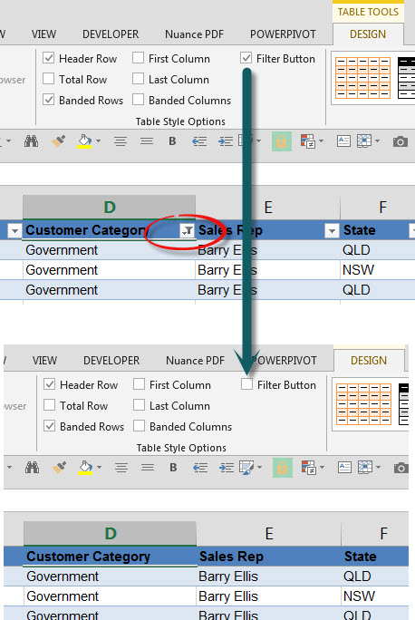
If you have used the Format as Table option on a table you now have the ability to turn off the filter icons in the header row without losing the filter that has been applied.
The new Option is in the Table Style Option section of the DESIGN ribbon, see image below.
The New Slicer in Excel 2013
Slicers are a graphic filtering tool added in Excel 2010. They allow you to filter Pivot Tables. Excel 2013 added a new slicer that makes filtering by dates a lot easier.
Summing Coloured Cells in Excel
A SUBTOTAL trick worth learning
In my training sessions I sometimes get asked about summing cells based on their colour. A SUMIF based on colour.
Excel and Hyperlinks
Sometimes you want them, sometimes you don't
Hyperlinks are a great tool as they allow you to speed up and simplify navigation within a file. Sometimes hyperlinks can be frustrating. See how to remove some of those frustrations below.
Protecting Your Excel VBA Macro Code
Applying a password to VBA
The more you use macros the more important they become and the more you want to make sure the VBA* code doesn’t get changed by someone who shouldn’t change it. You may also want to stop people viewing your code.


