Filtering Tables in Excel 2013 with Slicers

Sometimes when you apply a filter to a table it isn’t obvious what filter has been applied. This is the case when you are filtering by multiple entries in a field.

Slicers were introduced in Excel 2010 to filter Pivot Tables. Filtering a Pivot Table has the same issue when filtering by multiple criteria in a single field. Click here to see a post on these Slicers.

Slicers’ abilities were expanded in Excel 2013 to include filtering formatted tables. (A formatted table is one created using the Format as Table icon on the Home Ribbon tab or the Table icon on the Insert Ribbon tab).

The advantage with using a Slicer is that it is visual. It shows the filter being applied. A normal filter is hidden once selected.

The disadvantage with Slicers is the filters are limited to selecting or deselecting entries in the list. There is not the flexibility provided by Excel‘s normal filtering options.
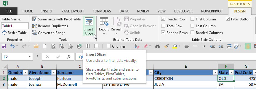
Adding a Slicer

In the Design Tab when a formatted table is selected there is an Insert Slicer icon.

Insert Slicer icon

A dialog displays allowing you to select fields to add Slicers.

Slicer selection dialog


Slicer added

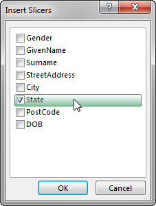
To select multiple items hold the Ctrl or Shift keys whilst clicking the entries.

Slicer Filter applied

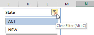
As you can see the Slicer shows the states being filtered.

To clear the filter click the icon on the top right of the Slicer.

Clear filters

Excel Hyperlink on a Logo

Using images for hyperlinks

In some files there is a central sheet that you keep returning to. It might hold the inputs or the controls for the file. You can simplify getting to that sheet by using a logo as a hyperlink.

Using a logo means you can place it anywhere on another sheet. It’s also easy to copy and paste the logo on other sheets once created.

You can add a hyperlink to any image, so it doesn’t have to be a logo.

There are two easy ways to open the Insert Hyperlink dialog.

Either right-click the image and select Hyperlink – see image below.

Right click Menu

Or select the image and press Ctrl + k.

Click the Place in This Document button and select the sheet to go to. You can also link to a named range. They would be listed under Defined Names. Using a range name avoids sheet name changes that can break hyperlinks.

Iisert Hyperlink dialog

Click OK and it’s done.

Useful Shortcut – return from hyperlink

After you follow a hyperlink you can return to where you were when you clicked it by first pressing F5 and then pressing Enter.

Stay tuned for a way to create an almost unbreakable hyperlink in a future blog post.