You can use conditional formatting to insert symbols in cells. You can also use formulas with emojis. using range names makes it even easier.
To insert an emoji icon in a cell you can use press the Windows key and the full stop.
This opens the Emojis dialog box.
In this example we are going to insert three separate symbols in formulas.
I have named each cell that has an emoji. A1 = Tick, A2 = Cross and A3 = Dash.
You can use these names in formulas throughout the file.
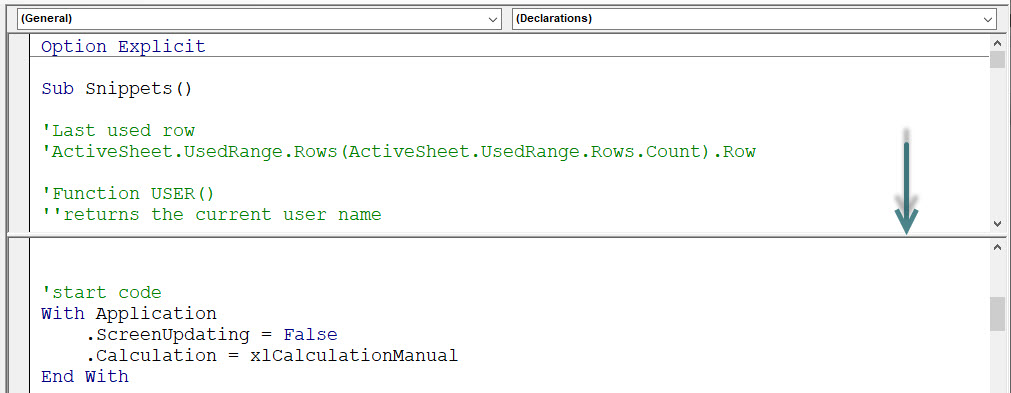
The formula in cell F2 (Sales) is.
=IF(D2>E2,Tick,IF(D2<E2,Cross,Dash))
The formula in cell F3 (Costs) is.
=IF(D3<E3,Tick,IF(D3>E3,Cross,Dash))
The advantages with using formulas instead of conditional formatting is that you can format the cells. Plus using formulas in cells is easier than using formulas in conditional formats.
Naming your emojis makes then easier to use. You can use these emoji icons names in your formulas throughout the file.
The typical range reference looks something like A1:A10. You always refer to the top left cell followed by the colon followed by the bottom right cell of the range. Did you know Excel can handle you entering the last cell followed by the first and it corrects it for you?
Clear all formats
To clear all the formats for a cell or a range select the cell/range and press in sequence Alt H E F don’t hold the keys down.
All the formats will be removed.
If you need to see the underlying number for a date this is an easy way to find it.
Laptop keyboards tend to re-purpose function keys to handle other features. Often the default for the function keys is the laptop features. You then must press the Fn key to access the software function key options. Look out for a FnLock option.
Did you know you can use Emojis on the sheet tabs? The font on sheet tabs is small, so some emojis may not be that effective, but simple emojis can be.
Excel Sparkline charts don’t have a horizontal axis. Here is a technique that creates one in the cell above or below the Sparkline. This works best for the Column Sparkline.
Sometimes with Excel formatting you just want to clear everything and start again from scratch. You can clear just the formats, and there is an icon you can add to the Quick Access Toolbar to make clearing all the formats earlier.
Excel allows you to easily hide and unhide rows and columns using a feature called grouping. There are two keyboard shortcuts that allow you to apply and remove grouping. These shortcuts can also be used to amend existing groupings.
Applying a date format before you drag with the Fill Handle may save you some time. See why.
Drop Down Selection update
Woohoo!
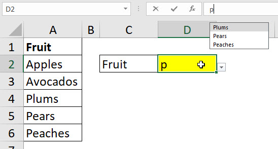
It has taken a decade or so but Excel finally has an in-cell drop down that you can type a letter and reduce the entries listed – see screen shot below.
Excel Has Ordinals
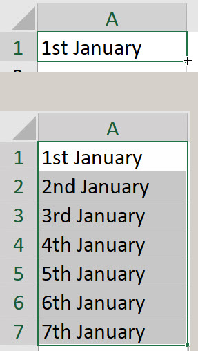
Woohoo, I don’t know when this happened, but you can now get Excel to extend your ordinals when you drag with the Fill Handle and use things like 1st, 2nd, 3rd and 4th etc.
Type 1st January in a cell and drag the cell down.
It seems to work with ordinals at the start rather than at the end of a text string. So January 1st doesn’t work. 1st by itself does work.
Excel’s new TEXTBEFORE function simplifies extracting text from the left. In this example I share how to extract all the text before a number in a code.
A client recently requested a formula to round to the nearest 9 cents. This avoids getting to a price point. This is a common requirement in retail businesses. The solution was simpler than I thought it would be.
Open Power Query Shortcut
Woohoo ! A new shortcut to open the Power Query window.
Works in the latest subscription version of Excel.
If you have the subscription version of Excel then you have access to the Navigation Pane. This allows you to navigate between sheets and see the structure of the sheets in your file.
In Excel you can use the Go To Special dialog to find constants. These are cells that won’t change. Constants are things like labels, entered text, numbers, or dates. But there are cells that won’t change that Go To Special won’t identify as a constant.
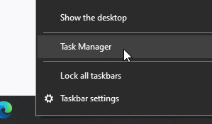
Task Manager
Wow – if you right click the Taskbar (bottom of the Windows screen) you can access the Task Manager.
Text alignment in Excel is versatile. If the column isn’t wide enough to display the text, it will display over the next cell. Date and number alignments are not so forgiving. If the column isn’t wide enough the cell with display the ### symbols or the scientific format. Here is a function technique to get around the limitation.