Grouping of dates in Excel’s PivotTables is fairly common and in the most recent versions of Excel, automatic. Many people don’t realise that you can perform other types of grouping in Excel.

The PivotTable below has five states listed.

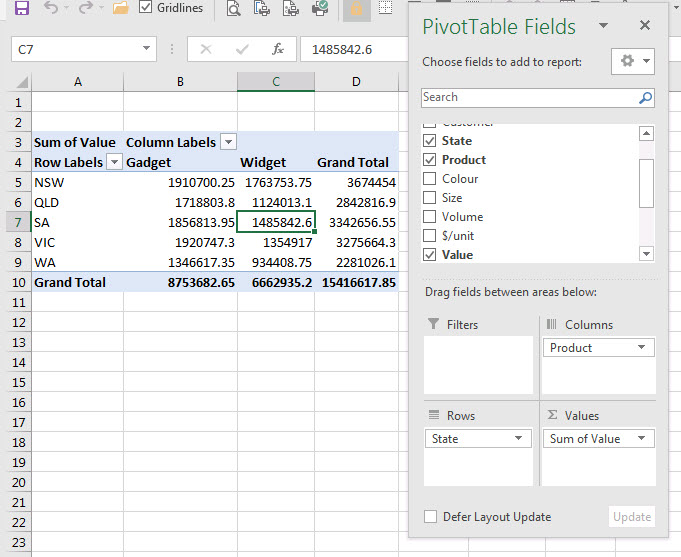
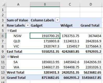
Let’s assume we want to categorise NSW, QLD and VIC as the eastern states and WA and SA as the western states.

The data does not have those categories built into it, but we can amend the PivotTable to create those groupings.

Ctrl key selection

You can hold the Ctrl key down and use the mouse to select multiple cells. We will use that technique to create the groupings in the PivotTable.

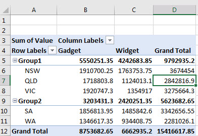
With the Ctrl key held down click the cells A5, A6 and A8. Right click one of the selected cells and choose Group.

Note the report will change as shown below

With the Ctrl key held down this time click the cells A10 and A12 from the image above (the indented SA and WA cells). Right click one of those cells and choose Group.

The PivotTable should look like the image below.

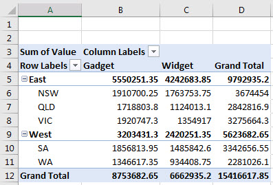
You can replace the generic Group1 and Group2 with descriptive names – just type in the cells – as shown in the image below.

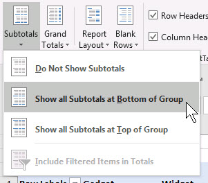
If you would like to show the totals at the bottom you can click the Design tab and choose the Subtotal drop down option (far left) shown below.

This changes the report as shown below.