Excel has a few counting functions. But when it comes to counting entries in a cell it can be difficult if you are using formulas that return a blank cell. This is where the SUMPRODUCT function can come to the rescue.

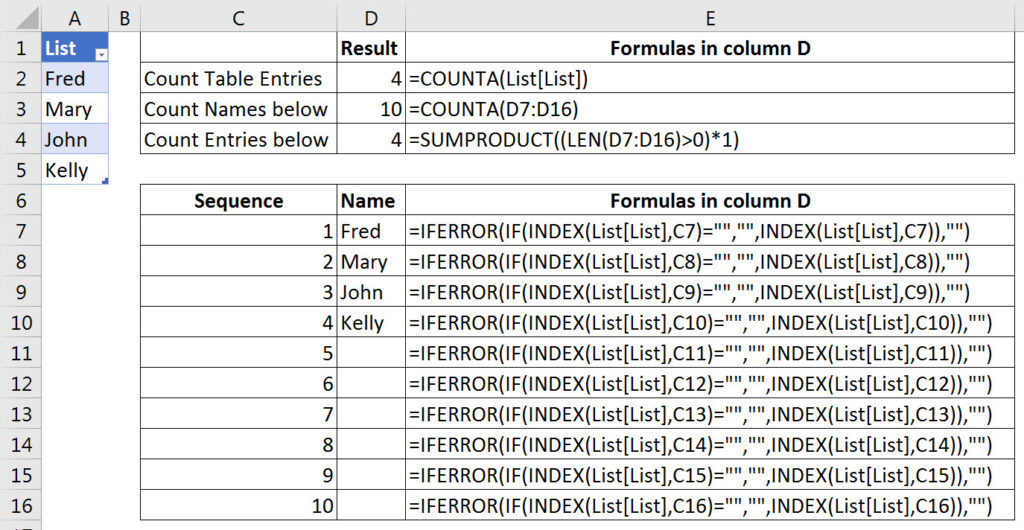
Have a look at the image below. The formatted table on the left-hand side has been named List. The example file can be downloaded via the button at the end of the post.

All the formulas in column D are shown in column E.

Column E contains the FORMULATEXT function which displays a formula from another cell.

The COUNTA function counts all entries.

Note: the COUNT  function (not shown) only counts numbers and dates.

Cell D2 counts how many entries are in the formatted table. This works well when the range contains only data entries.

In the listing that starts at row 6 I have used the INDEX function to extract entries from the formatted table based on the sequence number in column C.

The formula I have used identifies if a cell is blank. If a cell is blank it will display a blank. I am also handling more entries that the table currently contains so the IFERROR function will return a blank cell if an error is encountered. This means either an entry will be displayed or a blank cell with be displayed.

When we try and count the range D7:D16 the COUNTA function counts formulas as entries and displays 10. Even though the formulas are returning a blank cell they are still counted.

The formula to count cells that display entries is shown in D4 and it uses the SUMPRODUCT function to calculate all of the entries that have at least one character.

SUMPRODUCT

The SUMPRODUCT function is Excel’s most flexible function because you can use other functions within its brackets and in doing so allow those other functions to refer to ranges.

Normally that LEN function (which stands for length) can only work on a single cell. But when you use the LEN function within the brackets of the SUMPRODUCT function you can refer to a range.

The LEN function returns the number of characters in a cell entry.

The SUMPRODUCT function works like an array function (an advanced excel formula technique) and it will return multiple results which are then analysed to return a single value.

In this case the length of all of the cells in the range D7 to be 16 are calculated and then compared to 0.

The formula

LEN(D7:D16)>0

This part of the formula returns TRUE for each cell in the range if the cell length is greater than zero and FALSE if it equals zero.

In Excel TRUE equals one and FALSE equals zero. The *1 on the end of the formula converts the TRUE into one and the FALSE into zero.

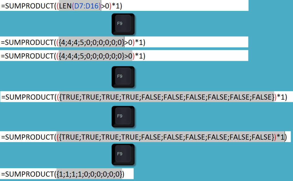
The SUMPRODUCT function then adds up those results to calculate how many entries in the range have a length greater than zero. You can see how this works below.

F9 function key

The F9 function key can be used to calculate part of a formula. When you are using it you need to make sure that the part of the formula you are selecting is able to be calculated independently. If you miss bracket then that can affect Excel’s ability to calculate and Excel will display an error message when you press F9.

In the image below I have selected parts of the formula and then pressed F9. You can see the results.

You can see that the length of each of the cells has been returned.

I then extend the area to include the >0 and press F9 again and you can see the TRUE and FALSE results based on comparing the lengths above to zero.

Finally when I include the *1 on the end you can see the TRUE and FALSE results converted into ones and zeros.

These are the amounts that the SUMPRODUCT uses to achieve its count result.

After using the F9 key you need to press Esc otherwise the values remain in the formula. You can Undo if you forget to press Esc.

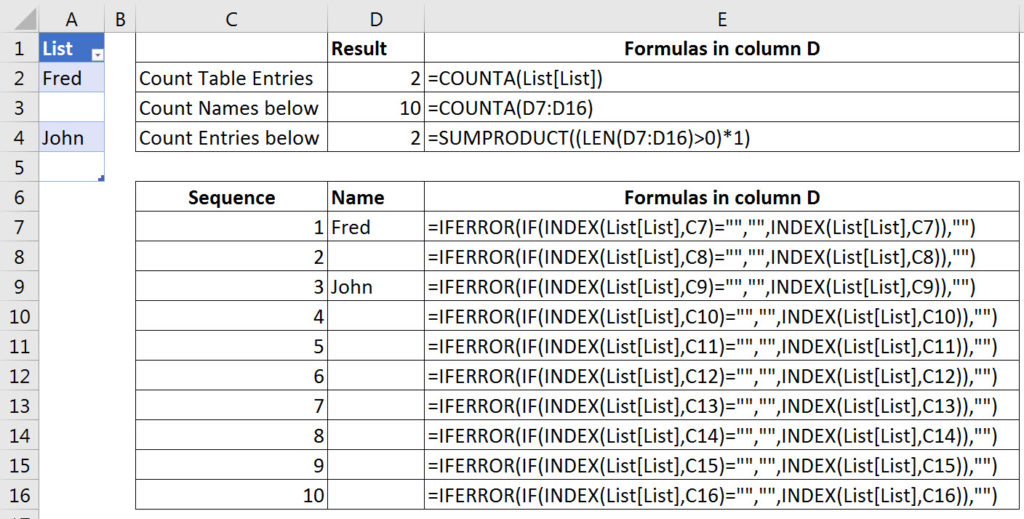
If I delete a couple of entries in the table you can see the results below.

Download Example File