There is a complicated way to extract the entries from a slicer but there is also an easy way to do it.
Slicers are filter interfaces that work with PivotTables and formatted tables.
In this example I will show you how you can find out what has been selected in a slicer for a PivotTable. You can download the example file using the button at the bottom of the post.
The technique takes advantage of the fact that the slicer can control more than one PivotTable.
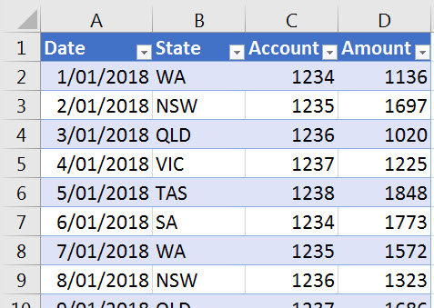
In the image below we have a basic data set that we will create a PivotTable from and then add a slicer for the State field (column) and then identify what has been selected from the slicer. The table is in a sheet called Data.
In the image below I have created a basic PivotTable that uses the data from above. This is in a sheet called Report.
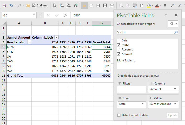
We can now insert a slicer to filter the state column.
One of the advantages of slicers is that you have the ability to filter by a column and also report on the column in the PivotTable. Using the Filter section of the PivotTable Fields dialog doesn’t allow you to both filter and report on a field (column).
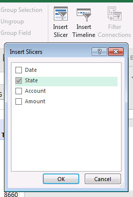
The Insert Slicer icon is on the Analyze tab when the PivotTable is selected.
The slicer is a graphical filter interface that allows you to filter a PivotTable by simply clicking the buttons.
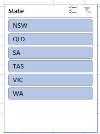
You can also hold the Ctrl or Shift keys to select multiple buttons. There is an icon at the top of the slicer that allows you to multi-select without having to use the Ctrl or Shift keys. The icon in the top right of the slicer clears the filters.
We are now going to create another PivotTable based on the same data sets but this time we are only going to list the states. This is also an easy way to identify unique values in a column. This is in a sheet called List.
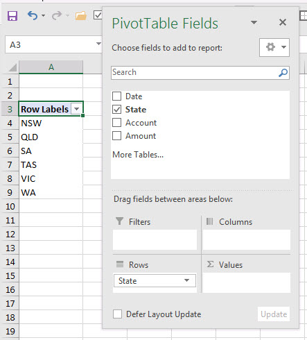
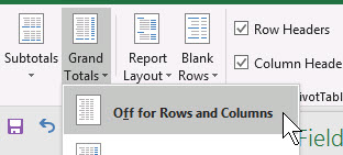
Note: I have removed Grand Totals from this report so only the states are listed.
Slicers have the ability to filter multiple PivotTables via their Report Connections option and we will use that to identify the entries that have been filtered by the slicer.
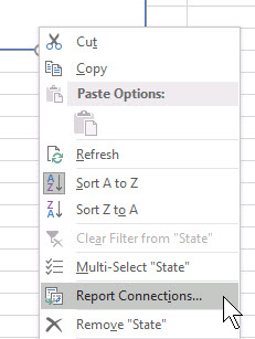
Right click the slicer on the original report and click the Report Connections option
This displays a listing of the other PivotTables that use the same data set. We can tick the other PivotTable and click OK.
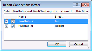
Now that both PivotTables are linked to the single slicer we can use the PivotTable we created in the List sheet to identify which states have been selected.
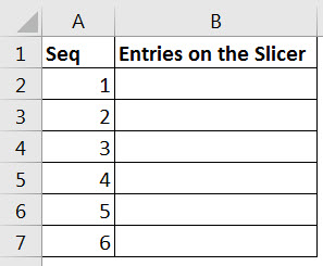
There are six states in our data set and on a separate sheet I will create a table that will extract the filters states from the pivot table in the lists sheet.
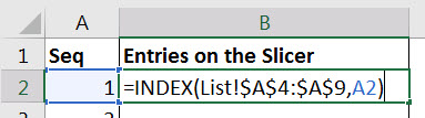
The formula for cell B1 is
=INDEX(List!$A$4:$A$9,A2)
This can be copied down the remainder of the table.
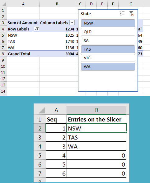
Any filters applied by the slicer will be reflected in the formula-based report. See the screenshots below.
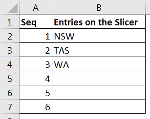
If you didn’t want to display the zeroes at the bottom of the formula-based list you could use the following formula.
=IF(INDEX(List!$A$4:$A$9,A2)=0,"",INDEX(List!$A$4:$A$9,A2))
This has been applied to the table below.
You could use this formula-based table as the basis for charts or reports that are all driven by the single slicer.
You may be asking – Why use the second Pivot when first Pivot has the States listed? Two reasons
- We didn’t want to have to handle Grand Total line – we could, but it would make the formula more complex.
- The original Pivot report layout may be adjusted, so having a second standalone Pivot ensures the layout doesn’t change.
Please note: I reserve the right to delete comments that are offensive or off-topic.