Excel’s HYPERLINK function is not easy to use. You need to know a few of its secrets to get it to do what you want. Unfortunately, you can’t replicate the HYPERLINK function in a custom function, so we can’t improve it. But the next best thing is to simplify creating the reference you need as the first argument in the HYPERLINK function.
Tag Archives: hyperlink
Hyperlink to a Specific Cell in Excel
Range name to the rescue
When you create a hyperlink manually in Excel it captures the cell reference. If you insert rows the cell reference in the hyperlink doesn’t update. If you need it to update, this is what you need to do.
Hyperlinking to a Cell in Another Excel File
It is possible
You can create a hyperlink to another Excel file in Excel but you can’t control what sheet or cell will be active. Well you can actually, but you need to know how.
Excel has Icons
New feature
If you have the subscription version of Excel, check out the Insert tab – you have Icons!
Hyperlink to a Range in Excel
Select a range with a click
Hyperlinks are a great way to navigate around complex spreadsheets. Most times when you create a hyperlink you link to a single cell within the sheet. In some cases there is a good reason to link to a range.
Creating a Hyperlink in Excel Based on a Search
Teleport to a cell in a data table
Let’s say you have a table of codes and every month there are a few you want to check out. You could use a VLOOKUP to extract all the details for each code, but let’s say you want to view the codes in the table.
Flexible Hyperlinks in Excel
Using the HYPERLINK Function
Hyperlinks are a great way to navigate around large spreadsheets. Unfortunately they each take a few clicks to create and can be easily broken. You can use a function to easily create multiple, flexible hyperlinks.
Getting Excel to Recognise an Email Address
Converting it into a hyperlink
Sometimes when Excel imports email addresses they are not recognised as emails and are not hyperlinks. They are two ways to fix this.
Excel and Hyperlinks
Sometimes you want them, sometimes you don't
Hyperlinks are a great tool as they allow you to speed up and simplify navigation within a file. Sometimes hyperlinks can be frustrating. See how to remove some of those frustrations below.
Excel – Unbreakable Sheet Hyperlink [VIDEO]
Changing a sheet name and deleting the hyperlink cell are two processes that can break Excel sheet hyperlinks. The video is at the bottom of the page.
Excel Hyperlink on a Logo
Using images for hyperlinks
In some files there is a central sheet that you keep returning to. It might hold the inputs or the controls for the file. You can simplify getting to that sheet by using a logo as a hyperlink.
Using a logo means you can place it anywhere on another sheet. It’s also easy to copy and paste the logo on other sheets once created.
You can add a hyperlink to any image, so it doesn’t have to be a logo.
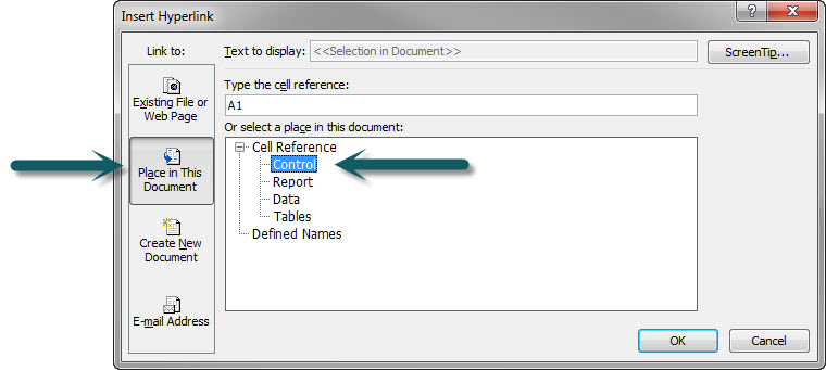
There are two easy ways to open the Insert Hyperlink dialog.
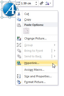
Either right-click the image and select Hyperlink – see image below.
Or select the image and press Ctrl + k.
Click the Place in This Document button and select the sheet to go to. You can also link to a named range. They would be listed under Defined Names. Using a range name avoids sheet name changes that can break hyperlinks.
Click OK and it’s done.
Useful Shortcut – return from hyperlink
After you follow a hyperlink you can return to where you were when you clicked it by first pressing F5 and then pressing Enter.
Stay tuned for a way to create an almost unbreakable hyperlink in a future blog post.

