Would you like to change the format of all your formula cells so they have a different fill colour or font? There is a way in Excel 2013 onwards.

In Excel 2013 a new function was added called ISFORMULA. This function enables you to identify formula cells. It returns TRUE if a cell contains a formula. In Excel all formulas begin with the = sign. Combine this with Conditional formatting and you can create a rule to format formula cells.

1. Select the range to work on.
2. Click the Conditional Formatting icon drop down and choose New Rule.
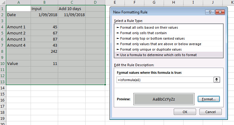
3. In the Dialog that opens click the last option in the top section (Use a formula to determine which cells to format) and enter the following formula in the box

   =ISFORMULA(A1)

   The cell reference needs to be the cell in the top left corner of the range you have selected. Make sure it doesn’t have any $ signs in the reference.

   
   The formula must return TRUE for those cells you want to format. The ISFORMULA function returns TRUE for formula cells.

4. Select a format using the Format button – in the above dialog I have used a mid-grey fill colour. Click OK.

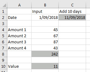
Cell B10 is formatted because it has this formula

=5+6

Formulas start with the = so even though this cell’s value won’t change it is included as a formula because it starts with the = sign.

Any new formulas will be automatically formatted.