In my training sessions I sometimes get asked about summing cells based on their colour. A SUMIF based on colour.
There isn’t a built-in function that handles it but you can use the SUBTOTAL function in combination with filtering to achieve the result.
(Note: another solution is to use a User Defined Function (UDF), but that is an advanced topic.)
The SUBTOTAL function has the ability to perform calculations based on visible cells only. When you combine that with Excel’s filtering feature that can filter by colour, you can sum up the filtered rows to achieve the result.
Filtering by colour is a recent addition to Excel’s feature set. It was added in Excel 2007.
This list has two t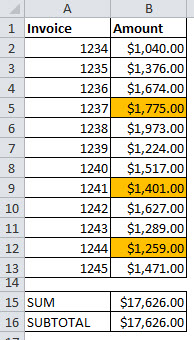 otals at the bottom.
The first uses a standard SUM function and the second a SUBTOTAL function that ignores hidden cells.
The formula in B16 is
=SUBTOTAL(109,B2:B13)
Normally 9 is used to define the SUM function calculation, but 109 instructs Excel to perform a SUM and ignore hidden cells.
If we right click one of the orange cells we can select Filter and then Filter by Selected Cell’s Color.

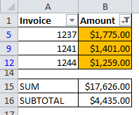 The list is now filtered and as you can see the SUM function hasn’t changed, but cell B16 has.
It shows the total for the orange cells only.
Using 109 in the SUBTOTAL can be handy if you have a sheet with hidden rows and you are wondering if there are values in those hidden rows. You can compare a SUM and a SUBTOTAL with 109 to see if they provide the same result.
Please note: I reserve the right to delete comments that are offensive or off-topic.