If you need to find the highest or lowest three entries in a filtered list you can use the AGGREGATE function to find them.
The AGGREGATE function was introduced in Excel 2010. It works in a similar way to SUBTOTAL It has the ability to make calculations based only on visible cells. This means you can apply a filter to a list and then perform a calculation on that list based on the visible cells and ignore the hidden cells.
You can download the example file at the button at the bottom of the post.
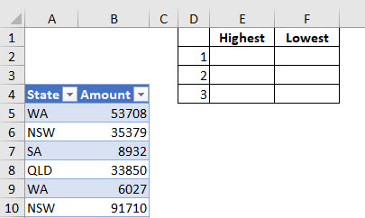
In the example below we have a list of states and values and we will find the top and bottom three values when the list is filtered by state.
The AGGREGATE function allows you to select a function (calculation) and then an option to determine the type of cells to ignore.
Note the AGGREGATE function only works on columns of data – vertical data. It won’t work on rows of data going across the sheet – horizontal data.
Syntax
AGGREGATE(function-num,options,array,k)
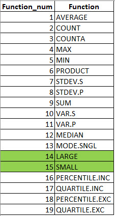
function_num – this is a number that identifies the function to use for the calculation. Below is a table of all the functions. We will use the two highlighted functions in this example.
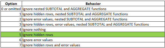
options – this is a number that specifies the type of cell to ignore when performing the calculation. A table of the option numbers is shown below. The highlighted option is the one we will use in this example.
array – this is the range to use in the calculation.
k – this is optional – it is only used if the selected function requires an extra argument. We need to use it in our example.
Note: the AGGREGATE function only works on columns of data (vertical data). It doesn’t work on horizontal data.
The formula for cell E2 is
=AGGREGATE(14,5,tblStates[Amount],D2)
This can be copied down. Column D has the helper cells that enable the copy down.
This uses the LARGE function and ignores hidden rows. The LARGE function allows you to extract the largest, second largest and third largest values by using a number to identify the position. 1 is the largest; 2 is the second largest etc.
The 5 in the formula instructs Excel to ignore values in hidden rows. It doesn’t matter how the rows were hidden they will be ignored. They could be hidden via a filter, a grouping or the hide rows option.
This formula is using a structured reference for the range. This refers to the formatted table’s column. The table in column A and B is a formatted table. The table has been named tblStates and the column name is Amount, which is enclosed in square brackets to identify it as column.
You can learn more about formatted tables and their advantages at the two blog posts below.
The formula for cell F2 is
=AGGREGATE(15,5,tblStates[Amount],D2)
This can be copied down. It uses the SMALL function and ignores hidden rows.
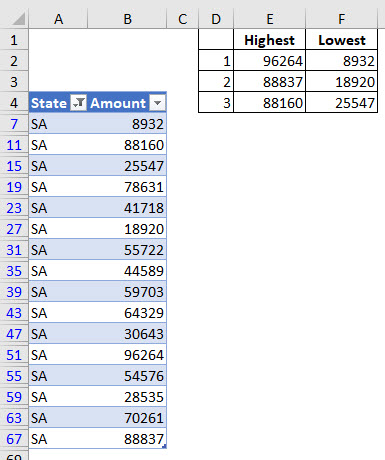
When you apply a filter to the data in columns A and B the formulas in columns E and F will update. Examples below.

Please note: I reserve the right to delete comments that are offensive or off-topic.