There are a couple of techniques to automate a unique list of items in Excel. I have covered them in previous blog posts (see links below). I thought I would describe how to use Power Query to create a dynamic unique list.

You can use a Pivot Table to create a unique list – the problem is that it is difficult to create a dynamic range name from the PivotTable.  I discussed the PivotTable solution at the button link below.

PivotTable Example

You can also use the Advanced Filter to extract a unique list. The issue here is that you need to re-apply the filter to update the list. You can read about it in the button link below.

Advanced Filter Example

I also suggested a UNIQUE function in Microsoft Uservoice – you can vote for it at the button below.

Vote for UNIQUE Function Example

Power Query Solution

Power Query gets around the above issues. Using Power Query to solve this issue is a bit like using a sledge hammer to crack a walnut but it shows how easy Power Query can be to use.

Our source data is in a formatted table named tblStates.

You can download the example files (before and after) at the links at the bottom of the post.

(See this post on formatted tables if you don’t already use them).

The State column could have new states added. We want to extract a unique list of states from the table so we could use them in a drop down list and a summary report.

Power Query Steps

1. Click anywhere in the tblStates table.
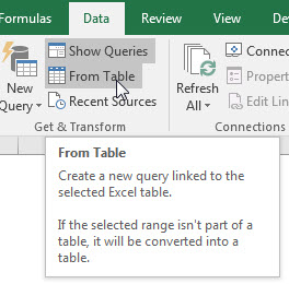
2. Click in the Data ribbon tab. In the Get & Transform section click the From Table icon.
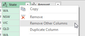
   If you have Excel 2010 or 2013 the icon is in the Power Query ribbon tab.
3. In the Power Query window that opens up right click the State column and Choose Remove Other Columns.
   This means if other columns are added to the data table they will be automatically removed. Leaving just the State column.
4. Right click the State column and choose Remove Duplicates.
5. On the right-hand side of the window rename the query to tblStates_New.
6. Click the Close and Load icon.

A formatted table is created with a list of unique states.

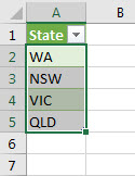
We can use the formatted table as the source for a range name to allow us to create drop down lists and a report.

Range Name Steps

1. In the newly created table select the range A2:A5 and click the Formulas ribbon tab
2. Click the Define Name icon.
3. In the Name section at the top, enter States and click OK.

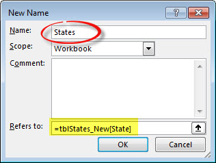
You may have noticed that the reference at the bottom (coloured yellow above) of the New Name dialog referred to the new table. Because this refers to the table reference it will automatically expand as new data is added to the table. This naming technique has lots of applications.

To update the unique list all you need to do is to press Ctrl + Alt + F5, which is the keyboard shortcut to Refresh All.

If this shortcut doesn’t work then check out this Tips post which describes a problem with Intel graphic cards that can cause a conflict for this particular shortcut.

If we add another row to the bottom of the initial table and create a new state, say TAS. To update our report and our drop down list you press Ctrl + Alt + F5.

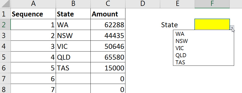
In the Report sheet in the file I have created a simple report that refers to the list that we just created – see above image.

The formula in cell B2 is

=IFERROR(INDEX(States,A2),"")

This has been copied down and uses the INDEX function and helper cell to provide a list of states based on the range name.

Cell C2 has a SUMIF formula based on column B

=SUMIF(tblStates[State],B2,tblStates[Amount])

in cell F2 I have created a Data Validation drop down list that uses the range name. The data validation dialog for the cell is below.

If you wanted to have a sorted unique list you can modify the query.

Select a cell in the unique table, the query name should appear on the right of the screen – double click it to edit it. (If you added TAS then it will have 5 rows loaded)

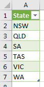
In the Power Query window click the filter drop down on the State column and choose Sort Ascending.

Click Close and Load and now the list will always be sorted when it gets refreshed.

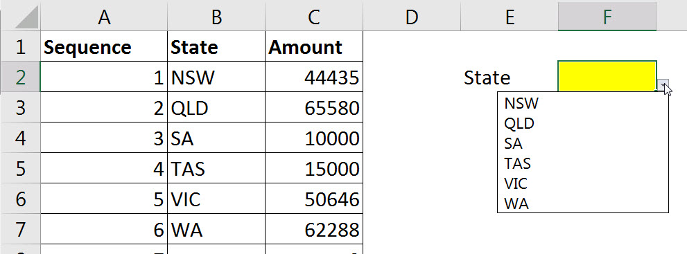
Add SA to the original table and press Ctrl  Alt + F5 and see the result.

The Report sheet is also updated.

Download example files below

Unique_PQ_before

Unique_PQ_After