Excel doesn’t have a MINIF or a MAXIF function and many advanced users create an array formula to provide that functionality. If you have Excel 2010 or later there is a non-array solution.
The AGGREGATE function was added in Excel 2010 and, like SUMPRODUCT, it can work with arrays without being array entered. The AGGREGATE function can also do something no other function can do. It can ignore errors, an important part of the solution below. You can download the example file at the bottom of the post.
Arrays are special formulas that must be entered in a special way by pressing Ctrl + Shift + Enter (often shorten to CSE). This places braces { } around the array formula. Array formulas can create very advanced calculations that can work through all the cells within a range to extract an answer. Most users are unaware of arrays and how they work.
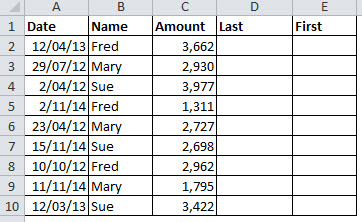
The AGGREGATE function, like the SUBTOTAL function, can perform many types of function calculations. In this case we will use it on the data below to determine the first and last dates in column A for the names in column B.
The formula for cell D2 which will determine the last date for Fred is
=AGGREGATE(14,6,($A$2:$A$10)/($B$2:$B$10=B2),1)=A2
This creates a MAXIF calculation.
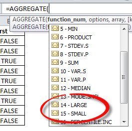
The 14 at the start specifies the function number for the LARGE function. See image below.
The 6 selects ignore errors, something only the AGGREGATE function can do – see image below.
We are purposefully going to create some errors that we want ignored.
The next part of the formula is normally where you would have a range, but in our case we have one range divided by another range. You can’t do this type of calculation in most Excel functions. Also the second range is not just a range but a range compared to a condition. This is where the MAXIF comes in.
($B$2:$B$10=B2)
This part of the formula will return a list of TRUE and FALSE results depending if the entry in column B equals Fred. See image below.
This was created by selecting $B$2:$B$10=B2 in the Formula Bar and pressing the F9 function key.
In Excel TRUE = 1 and FALSE =0. Hence when you divide the entries in column A by the corresponding TRUE (1) or FALSE (0) it will create divide by zero errors for each FALSE see image below, also created using the F9 key. Dividing by 1 (TRUE) leaves the numbers unchanged.
Dates are numbers in Excel and the numbers shown above are the three dates that match Fred. Now remember we have chosen the LARGE function (14) and ignore errors (6) so the errors will be ignored and those three number will be analysed by the LARGE function.
The last part of the AGGEGATE formula is 1. The 1 on the end here simply means you want the largest number. Using 2 would specify the second largest number.
So the errors are ignored and the largest number (date) is returned.
The final part of the formula compares the value returned by the AGGREGATE function to the date in column A. If they match, it will return TRUE, signifying it is the last date for the name in column B. If dates were duplicated there could be more than one TRUE for a name.
The formula for cell E2 which mimics a MINIF is
=AGGREGATE(15,6,($A$2:$A$10)/($B$2:$B$10=B2),1)=A2
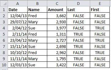
This is the same as the previous formula except for the use of 15 instead of 14 at the start of the function. 15 specifies the SMALL function. The final result is shown below.
If you had created a formatted table, the resulting formulas would look like these
MAXIF cell D2
=AGGREGATE(14,6,([Date])/([Name]=[@Name]),1)=[@Date]
MINIF cell E2
=AGGREGATE(15,6,([Date])/([Name]=[@Name]),1)=[@Date]
These are structured references that relate to the table fields and cells. They work like ranges names and I usually refer to them as table names.
Structured references automatically expand with the table. Formulas in formatted table automatically copy down and also all update when one is changed.
See a previous blog post on formatted tables here.


great!
Brilliant use of the AGGREGATE function! And a very well-written explanation.
Thanks Gabriel