If you need a formula to identify the last used cell in a column you don’t have to use an array formula. The AGGREGATE function can calculate it for you.

The AGGREGATE function was added in Excel 2010. It allows you to perform calculations that would normally require an array formula.

If you needed to find the last used cell in column A then the following formula will provide the result:

=AGGREGATE(14,6,ROW(A:A)/(NOT(ISBLANK(A:A))),1)

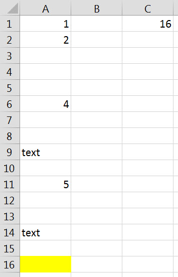
This formula is in cell C1 in the image below. Note: cell A16 which is highlighted yellow has an IF formula that returns a blank cell – but it is still identified as the last used cell.

The AGGREGATE function can perform different calculations, similar to the SUBTOTAL function.

The first argument in the AGGREGATE function determines the calculation to perform. 14 refers to the LARGE function. The LARGE function is like a flexible MAX function where you can specify whether you want to return the first, second or third highest value in a range. The ,1 at the end of the AGGREGATE function is instructing the LARGE calculation to return the highest value.

The second argument in the AGGREGATE function specifies whether or not to ignore subtotals, errors or hidden rows. Using the number 6 instructs Excel to ignore all errors.

ROW(A:A)/(NOT(ISBLANK(A:A)))

This part of the formula will return all of the row numbers that have an entry in them.

The row number itself is divided by a combination of the NOT function and the ISBLANK function. This combination will return TRUE when an entry is found in column A. The ISBLANK function returns TRUE when a cell is blank. But we want to identify non-blanks. That is why we use the NOT function with the ISBLANK function. The NOT function converts TRUE to FALSE and FALSE to TRUE.

The NOT-ISBLANK combination produces a series of TRUE and FALSE results. In Excel TRUE equals one and FALSE equals zero. So when you divide by TRUE you leave the row number unchanged. When you divide by FALSE you create a divide by zero error.

The trick to this technique is that by dividing by FALSE creates an error. So all the row numbers that are divided by zero will return an error. And the fact that we used 6 as the second argument in the AGGREGATE function means that the LARGE calculation will ignore all those errors. This leaves just the row numbers that have entries in them. The LARGE function will return the highest row number that has an entry.

You could use the above technique to get the last row numbers of cells that match a criteria as well.

Note: the AGGREGATE function only works on columns. It doesn’t work across the sheet on rows.