Slicers are a graphic filtering tool added in Excel 2010. They allow you to filter Pivot Tables. Excel 2013 added a new slicer that makes filtering by dates a lot easier.
Its called a Timeline slicer (see image below – you need to have a Pivot Table selected to see these options) and it makes filtering by months and quarters a lot easier. It was common in previous versions to add columns (fields) to your data to make filtering by months and quarters easier.
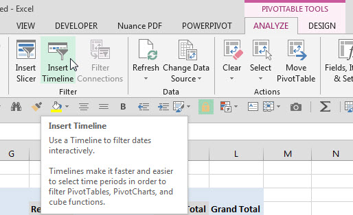
When you click the Insert Timeline icon it automatically identifies the date columns (fields) in your data, as per the image below.
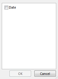
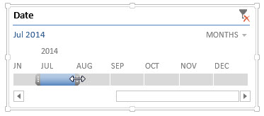
When you tick the Date field and click OK it will display the slicer.

You can click on individual month to display only that months. When you point to either end of the selection bar you can see a double-headed arrow which allows you to click, hold and drag to select more months.
The drop down option in the top right corner allows you to select Days, Quarters and Years. Note: quarters are calendar year quarters.
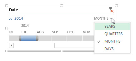
The icon with the red cross in the top right corner will remove the current filter.
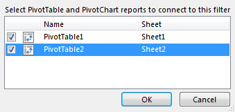
One Slicer can filter multiple Pivot Tables. Simply right click the slicer and choose Report Connections.

Tick the Pivot Tables you want to filter and click OK.
 You may be interested in these two other posts on slicers.
Please note: I reserve the right to delete comments that are offensive or off-topic.