Always Refer to Cell A1
If you need to ALWAYS refer to cell A1, regardless of whether row or columns are inserted or deleted, then use the following formula.
=INDIRECT("A1")
This will always display the entry in cell A1 on the current sheet.
Another formula that always refers to cell A1 on the current sheet is
=INDEX(1:1048576,1,1)
VBA Window Tip
To open the VBA window press
Alt + F11
This shortcut actually toggles between the Excel window and the VBA window – but if the VBA window isn’t open, it will open it.
Stop Text Being Input
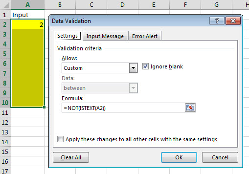
If you want to stop text being entered in a range you can use a Custom Data Validation formula.
Select the range and press in sequence, not held down, Alt a v v. This opens the Data Validation dialog.
From the Allow drop down select Custom (last entry).
In the Formula box enter the following formula
=NOT(ISTEXT(A2))
Replace A2 with the top left cell in your range. Make sure there are no $ signs in the reference.
Click OK.
Close Excel Quickly
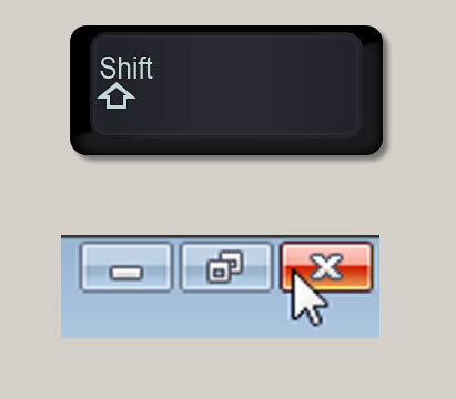
In the more recent versions of Excel, when you click the X in the top right corner, you only close the current file.
In the older versions this would have closed Excel down, and you could then save each file in sequence.
To get the same effect in the new Excel, hold the Shift key down whilst you click the X with the mouse.
If you want to save all the open files click here to see a blog post with a macro to do just that.
Print Titles
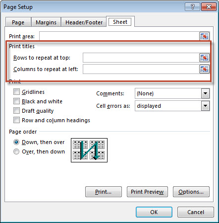
Print Titles is the term Excel uses to describe the rows and columns you want repeated when you print a sheet over multiple pages.
You typically want to repeat the labels in the top row(s) and those in the left column(s) of the sheet.
There is a dedicated button to define Print Titles on the Page Layout ribbon tab.
You can display multiple rows and columns.
Range Names List
If you use range names then it is a good idea to include a list of all the range names in a file for documentation purposes.
There is a shortcut that does all the work for you.
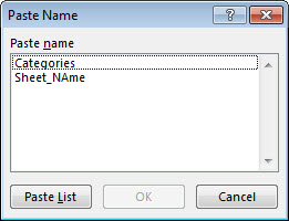
Select the cell where you want to enter the list.
Press F3 and then click the Paste List button.
The list has two columns. The range name and it’s reference.
The list is not dynamic. If you add, delete or change the names you will need to do the paste again.
Today’s Date
The formula that will always display today’s date is
=TODAY()
The keyboard shortcut to enter today’s date in the active cell as an input is
Ctrl + ;
The VBA line of code to enter today’s date in cell A1 is
[A1] = Date
Right Click – Filtering
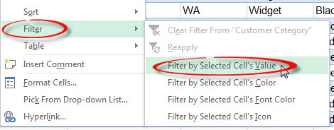
One of my favorite and frequently use right click tips is the Filter option.
You can click a cell within a table that contains the entry you want to filter by, then click the Filter option and then Filter by Selected Cell’s Value.
Note : you can also filter by font and fill colour.
Display a Ratio
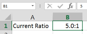
To have a value show as a ratio 5.0:1 you can use a custom number function.
The value in the cell is 5, but it displays as 5.0:1. This means you can still do calculations and comparisons with the value.
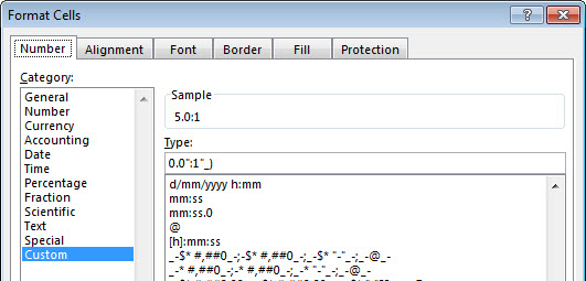
The format is
0.0":1"_)
Find Errors
Excel has seven error messages that can be displayed when something goes wrong with a formula.
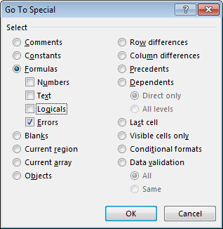
To find errors you can use the Go To Special dialog.
Press F5 then click the Special button.
Click Formulas and then uncheck Numbers, Text and Logicals. Click OK. See image below.
Now all the error cells are selected you could apply a fill colour at this stage to make then stand out.
To move between the selected cells press the Enter or Tab keys. DON’T use the arrow keys, as this will deselect the error cells.
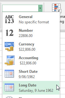
Day Of The Week
A quick and easy way to find out the day of the week for a specific date is to use the Long Date format from the drop down in the middle of the Home ribbon (in the Number section) – see below.
Returning a Blank Cell
You can’t use a formula to return a truly blank cell. It may look blank, but it isn’t.
Blanks cells are selected when you use GoTo Special Blanks.
Typically you want to convert cells containing only spaces into blank cells.
Note: this technique assumes the other cells in the range don’t have spaces.
You can select the range press Ctrl + h and type a space in the Find Box and click the Replace All button.
This converts all the cells with spaces into really blank cells.
Days in Month Formula
If you need to calculate how many days in a month, you can use two functions together.
Assuming cell A1 has a date within the month, you can use
=DAY(EOMONTH(A1,0))
Clearing the tab colour
I use colours on my sheet tabs to signify different things.
To clear a colour, you can use the following keyboard shortcut
Alt h o t n
Pressed in sequence, not held down.
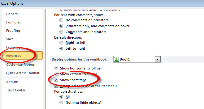
Show Sheet Tabs
If you find the sheet tabs are missing at the bottom of the screen, you can fix the issue with the setting below.
To access this screen press, in sequence (not held down)
Alt t o a
and scroll down about half way.
Clearing Filters
The keyboard shortcut to clear all filters is pretty straight forward
Alt a c
Keys are pressed in sequence, not held down.
Paste Values
After copying, use the following keyboard combination to paste just the values – no formulas or formats.
Alt h v v
These keys are pressed in sequence, not held down.
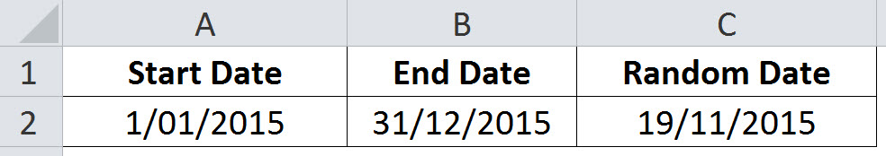
Random Dates
In Excel dates are stored as numbers.
To generate random dates you can use the RANDBETWEEN function with a start date and an end date.
=RANDBETWEEN(A2,B2)
Cell C2 has been formatted as a date.
This formula is dynamic. Each time Excel calculates it will update and most likely change.
You can use Copy > Paste Values to capture the date(s).
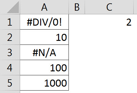
Counting Errors in a Range in Excel
If you need to ensure that a range has no errors you can count the errors and compare the result to zero to ensure the range is error free.
The formula in cell C1 which counts errors in a range is
=SUMPRODUCT(ISERROR(A1:A5)*1)
If you want to display TRUE for no errors and FALSE for error(s) you can use
=SUMPRODUCT(ISERROR(A1:A5)*1)=0
You can also use an IF function to display the text Error if any errors are found.
=IF(SUMPRODUCT(ISERROR(A1:A5)*1)=0,"OK","Error")
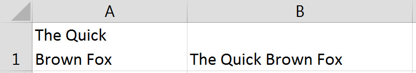
Removing Line Feeds in Excel
Sometimes when text data is imported from other systems it can contain line feeds.
A line feed wraps the text onto a new line – it is not associated with the Wrap Text format.
Cell A1 below shows an example. Cell B1 has the formula that removes line feeds and replaces it with a space.
The formula in B1 is
=SUBSTITUTE(A1,CHAR(10)," ")
Controlling the Enter Key
When you press the Enter key Excel typically selects the cell beneath the current cell.
Some people change this default option so that the selected cell does not move at all when Enter is pressed.
When you think about it, you often press Enter and then immediately move back to the cell to either copy it, or format it.
If you want to change what the Enter does when you press it, you can change a setting in Excel Options.
In the Advanced section of Excel Options (press Alt t o in sequence to see Excel options) the very first option controls the Enter key.
If you un-tick the option the Enter key will not change the selected cell when pressed.
You can see from the image above that you can also get the Enter to move in any of four directions.
Using the Right option may be handy if you are entering data across a page.
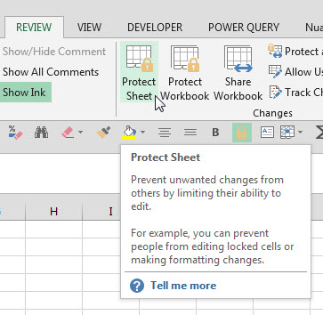
Easy Protection
Applying sheet protection stops your sheet structure from being accidentally changed by you, or someone else.
You can add sheet protection by right clicking the sheet tab and clicking Protect Sheet or using the Protect Sheet option in the Review tab.
You typically use a password when applying protection, but you can also leave the password box blank.
This still applies sheet protection and stops accidental changes, but allows you to easily unprotect the sheet; make a change and then re-protect your sheet without a password.
This stops accidental changes but allows for quick changes and you don’t have to remember a password.
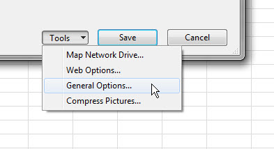
Backup your important files
Excel has a feature that has been around for many versions, but most users are unaware of it as it is tucked away in a separate menu and dialog.
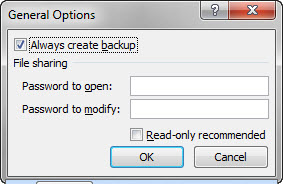
You can have Excel automatically make a backup of the previous version of a file each time you save it.
Note: if you click save twice in a row the backup will be identical to the current version.
This can be a life saver if your file gets corrupted.
In the Save As option (press F12 to open Save As) click the Tools drop down (left of the Save button) and choose General Options – see image below.
You may have to overwrite the existing file if you haven’t changed the name.
The file is saved as a .xlsb file – you can open it as per a normal Excel file.
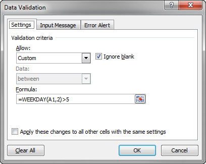
Data Validation to Ensure a Weekend Date
If you want to ensure the user enters a date that is a Saturday or a Sunday, you can use a Custom Data Validation.
This example is for cell A1.
To open the Data Validation dialog use Alt a v v (pressed in sequence, not held down).
Click the first drop down and select Custom. This allows you to enter a formula to determine the data validation.
The formula used is
=WEEKDAY(A1,2)>5
The WEEKDAY function returns a number from 1 to 7 for the days of the week. The ,2 in the function means 1 = Monday, 6 = Saturday and 7 = Sunday.
Click OK to apply.
If you wanted to ensure weekday dates you could use the formula
=WEEKDAY(A1,2)<=5
VBA AutoComplete
When you are typing code in the VBA code window you can press
Ctrl + Space Bar
to have Excel finish the word for you. Eg type
appli
And then press Ctrl + Space Bar to have Excel finish the word Application.
Counting Positives and Negatives
If column A contains positive and negative numbers, you may need to count how many of each. You can use the following two formulas.
Positives
=COUNTIF(A:A,">0")
Negatives
=COUNTIF(A:A,"<0")
Zeroes
There may be zeroes as well. The formula to count them is
=COUNTIF(A:A,0)
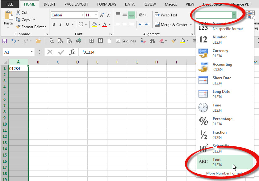
Inserting values that start with 0
To enter numbers that starts with a zero eg mobile telephone numbers, start with the single inverted comma ‘ then type the number and press Enter.
If you are going to enter a whole column of them, it may be easier to format the whole column as Text – see image below.
When you use the Text format you don’t need to use the inverted comma, just type the number.
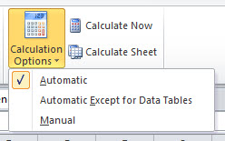
Calculation Warning
You have to be careful when turning off calculation in Excel. The calculation options are on the right of the Formulas ribbon tab – see image below.
Most people don’t turn off calculation and hence always expect the sheets to automatically calculate, so they may rely on the results even though they might not have been updated.
When you save a file and calculation has been turned off, the file remembers the calculation state and when you or someone else opens the file it will turn off calculation which again causes the previous issue
When you turn off calculation always remember to turn it back on (change to Automatic) before you save the file.
Space Bar Tips
To select the current column or columns hold the Ctrl key down and press the Space Bar. (Remember tip – Ctrl + column both start with c)
To select the current row or rows hold the Shift key down and press the Space Bar.
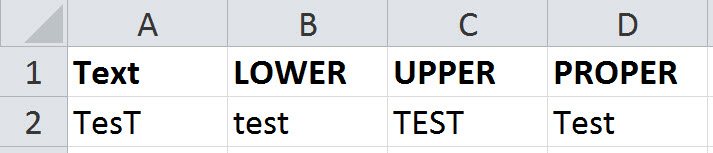
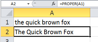
Grabbing the right case
Excel has three functions that handle case. LOWER, UPPER and PROPER.
See image below for the results of using these functions. Cell A2 contains an entry.
Cell B2 has =LOWER(A2)
Note: The PROPER function capitalises the first letter of every word in the cell – see below.