Range Selection Tip and Trick

You know how when you press Enter you usually select the cell below? You can override that without changing a single setting.

When you select a range Excel can behave differently when you press the Enter key. Not many users know this trick.

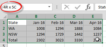
Select the range B2:G2 in a blank sheet and press Enter. The cell selected will be the one on the right or back at the start of the range depending which cell was active when the range was selected.

Pressing Enter cycles through all the cells in the range.

This works for two dimensional ranges as well – in that case the cell below is selected until the bottom of the range is reached then the top of the next column within the range is selected.

This is handy for entering data into input ranges.

Try This

Let’s say range A2:D2 has basic links referencing the cell above so cell A2 has =A1 in it.

What if you wanted to change all those relative references to fixed references?

Select the range A2:D2 and then press these three keys in sequence

F2 F4 Enter

Repeat three times – job done!

F2 is the Edit command.

F4 converts a relative reference into a fixed reference.

Enter accepts the change.

You can often achieve very fast changes with keyboard techniques like this.

For example if a cell contains an email address  or a web address but it isn’t recognised as a link, simply select the cell and press F2 then press Enter to convert it into a link.

If there is a column of them, just keeping pressing F2 and Enter to convert them all. You can become quite fast.

Marking cells Good-Bad-Neutral

Sometimes when you are reviewing a file against a printed report, you may need to identify when cell values are correct, wrong or close.

Consider using the built-in Styles Good/Bad/Neutral on the Home ribbon tab – see below.

These can be quicker than using the usual fill colour icon.

Remember they may not be useful for colour blind readers if you are sharing with other people.

Don’t forget once applied if you want to apply the same format to another cell press the F4 function key.

Once formatted you can sort or filter by colour – see right click options below.

Adding Values to Values

Let’s say you have an input cell that someone enters multiple values into eg

=10+5+34

You may have many such cells.

Now let’s say you want to add 20 to all these cells but keep the original values that have been entered in those cells.

Paste Special to the rescue.

1. Enter 20 in a blank cell and then copy the cell
2. Select the cells you want to amend – you can hold the Ctrl key down to select  multiple cells with the mouse
3. Open the Paste Special dialog
4. Click the options Values and Add – as per image below – then click OK – done!

The resulting formula will be something like

=(10+5+34)+20


Related Posts

					
			

				Drop Down Selection update
			
					
			

				Excel Has Ordinals
			
					
			

				Restarting Excel and Windows
			
					
			

				Open Power Query Shortcut
			
					
			

				VBA Window Split
			
			

Find and Replace Tips, Tricks and Traps

The keyboard short for Find is Ctrl + f.

For Find & Replace it is Ctrl + h.

Tips

Always, I mean ALWAYS, select the range you are working with before you run Find and Replace.

If you have a single cell selected it will affect the whole sheet – maybe not what you want.

Leave the Dialog Open

In the old days we used to close the Find dialog. Now you can leave it open if you need to change things in multiple files or sheets. You can navigate around with the dialog left open.

When using Find if you want to select all the cells it has found, click in the bottom section of the Find dialog where the cells are listed and press Ctrl + a this will select all the cells at once.

Number Formats

Be aware that sometimes numbers won’t be found due to formatting. eg if you search for 1000 but you have used the comma format eg 1,000 then the number might not be found.

You might need to do two Finds, with and without commas.

Formulas vs Values

Click on the Options button to see these options.

The default Look in: setting for Find (unfortunately) is Formulas. See image below.

This means if a formula returns what you are looking for it won’t be found. You need to switch this Look in: setting to Values.

Increase Decimal

I found a good shortcut today to increase the decimal places.

Alt H 0

For example you might use these two shortcuts one after the other to format a range as a percentage with one decimal place.

Ctrl + Shift + %

Alt H 0

Printing Separate Print Areas

If you need to print a number of separate print areas from the one worksheet in one step there is an option that allows you to create a print area that includes additional ranges.

Create your first print area as per normal.

Select another print range and click the Page Layout ribbon and use the Print Area drop down and choose Add to Print Area. Keep adding ranges as you require.

You can also use the Ctrl key and mouse to select multiple separate ranges and then use Set Print Area.

The above technique allows you to add to that Print Area if you miss a range.

Downside

The only problem with this option is that each separate range is printed on a separate page(s).

Close All Icon

If you have a lot of files open and you want to close them all and still leave Excel open you can add this icon to the Quick Access toolbar.

See this post if you are not sure about using the Quick Access Toolbar.

Sheet Protection – No password

When you protect a sheet with a password, you must make a note of the password, otherwise you create problems for yourself.

Did you know you don’t have to supply a password?

To apply sheet protection, right click the sheet tab and choose Protect Sheet.

When the Protect Sheet dialog displays just press Enter or click OK.

This protects the sheet with no password.

This stops accidental changes and you can easily unprotect the sheet to make changes.

You can right click the sheet tab to unprotect as well.

Format part of a text string

Many people don’t know that you can format part of a text string in a cell.

This can be useful if you want to highlight, or emphasis, a particular word or phrase in a text string.

You can double click a word in the Formula Bar or while editing in a cell and a small menu pops up – see image below.

The options are reasonably limited, but you can use Bold or Italic, change the font; the font size and font colour – see examples below.

Show or Hide Cell Comments

Cell comments (they are like a sticky notes for cells) are great for instructions and documentation.

To show all the comments press, in sequence, not held down

Alt r  a

This is a toggle, so you can use the same sequence to hide all the comments.

Note: Comments have been renamed Notes in later versions of Excel. Comments now refer to a new features of threaded comments.

Calculation Issue

There are two reasons your Excel file won’t calculate.

The first, and easiest to fix, is that Calculation is turned off – see a previous tip on that issue.

The other reason is that there is a Circular Reference in the file. Circular References can stop calculation.

You can confirm if there is a Circular Reference in a file by looking at the bottom left-hand corner of the screen – see image below.

A Circular Reference means that a cell is referring to itself in a calculation. A simple example is shown in the image above, where cell A1 has a formula =A1.

Excel cannot resolve this calculation, so zero is displayed.

In the Formulas tab, on the right-hand side, the Error Checking icon drop down will help you identify the Circular References in the file.

Turn on Calculation

The shortcut to turn on automatic calculation – pressed in sequence – is

Alt m x a

To turn it off

Alt m x m

Insert a New Sheet

To insert a new blank sheet press Shift + Alt + F1.

Open Paste Special Dialog

To open the Paste Special Dialog after copying or cutting use

Ctrl + Alt + v

WARNING: This conflicts with a default Evernote clipping shortcut. You can change it in Evernote use Tools > Options > Shortcut keys.

You Can Undo After You Save

I amazed how many people are unaware of a change that happened way back in Excel 2007.

In Office 2007 and later versions you can use Undo after you have saved the file.

In the old days (Excel 2003 and earlier) saving used to clear the undo list – it no longer does.

So undo to your heart’s content.

Remember there is a keyboard shortcut to undo.

Ctrl + z

Working with Quarters in Excel

You might not know that Excel knows about quarters. That’s 3 months, not 25 cents.

If you type Q1 in a call and drag the cell with the Fill Handle (bottom right corner of cell) you will see that Excel repeats the sequence Q1, Q2, Q3 and Q4. It doesn’t do Q5 or above.

This works for Qtr1 as well.

Selecting Ranges

When selecting a range with the mouse or keyboard, keep an eye on the Name Box – top left corner of the screen, just above the grid.

It tells you how many rows (R) and columns (C) you have already selected – see image below.

As soon as you release the mouse, or stop using the keyboard, the values will disappear. You have to be quick to see it.