Checking if entries are really the same

To check if two cells are the same you can use

=A1=B1

This returns TRUE if the values are the same or the text is the same ignoring case sensitivity.

In the above formula TEST will equal test.

To check if entries are identical, taking into account upper and lower case, then you can use

=EXACT(A1,B1)

In this case comparing TEST and test will return FALSE.

Formatting Pivot Tables

When formatting a Pivot Table is best to right click the values section of the report and choose Number Format.

PT_Format_tip

This will format the whole report, not just the selected range. Avoid using the Format Cells option as it only applies to the range selected.

How to Copy a Sheet

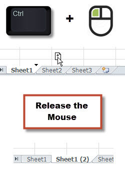
The easiest way to copy a sheet is to click and hold on the sheet tab name and then press and hold the Ctrl key down and move the mouse to where you want to paste the new sheet and release the mouse.

When you press Ctrl a small plus sign will display in the document icon to show it is copying, not moving the sheet.

Copy sheet

Close Existing File

To close the existing file you can use

Ctrl + w

If you want to save and close you can use on after the other.

Ctrl + s
Ctrl + w

The s and w keys are close to each other, so it can be a quick way to save and close a file with one hand.

Save and Close

Useful Formatted Table shortcuts

These apply to a formatted table (Format As Table icon used from Home ribbon – see below)

Table_tip
Ctrl + a Selects the table data – no headings

Ctrl + + inserts a new blank row in the table
Ctrl + – (minus) deletes a row from the table

Ctrl + Space selects all the data in a column – no heading
Shift + Space selects all the data in a row

The shortcut below works in any table formatted or not

Ctrl + * to select the table (use the * on the numeric keypad)

Copy As Picture

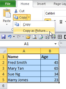
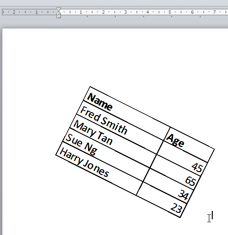
When copying between Excel and Word or PowerPoint, in some cases you may want to copy the range as a picture. This has the advantage of being easier to re-size and manipulate in Word or PowerPoint.

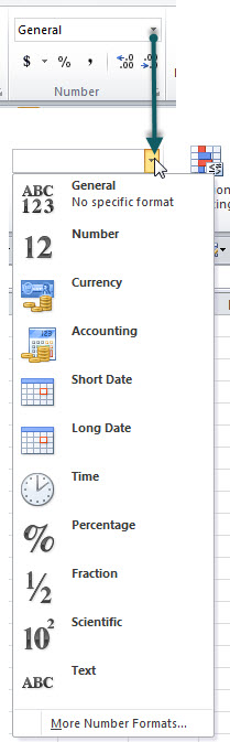
Select the range first and then use the drop down on the Copy icon on the Home ribbon – see below and select Copy as Picture

CopyAsPic_1
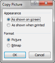
A dialog will display allowing you to specify the type of picture to create.

CopyAsPic_2
Click OK to accept the defaults

You can then paste into the other application and treat it like an image.

CopyAsPic_3

Excel 2013 Hide Filter Icon in a Table

This tip applies to Excel 2013 only.

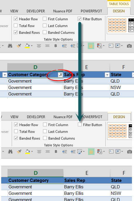
If you have used the Format as Table option on a table you now have the ability to turn off the filter icons in the header row without losing the filter that has been applied.

The new Option is in the Table Style Option section of the DESIGN ribbon, see image below.

Filter_1

Related Posts

VBA Functions

If want to see a list of the functions available in the VBA language just type

vba.

in the code window

VBA_Tip_1

You don’t need to include vba. when using the function in code.

If you see a function with a $ in its name it means it returns a string (text) eg UCase$

VBA_Tip_2

(Thanks to John Walkenbach for this tip.)

Click here to see how you can run a Macro off a Quick Access Toolbar icon.

Related Posts

Two Spaces

There are two types of spaces in Excel. The normal space and one that is called a non-breaking space, often found on websites.

When using some of Excel’s features Excel doesn’t recognise the other type of space. You can use the following formula to convert all non-breaking spaces in a cell to the normal space. Assume the text is cell A1.

=SUBSTITUTE(A1,CHAR(160),CHAR(32))

The CHAR function allows you to refer to ASCII characters by their number. 160 is the non-breaking space, 32 is the normal space.

This blog post discusses the CHAR function in more detail.

Automatic Drop Down List

Excel has a drop down list that is automatic. Check the image below

Tip_PickList

Things to note:

  • Cell A1 is bold – that tells Excel its a column heading.
  • I have entered two names, Fred and Mary
  • In cell A4 when you use Alt + down arrow Excel automatically displays the list of the entries from above.
  • You can use your arrow keys to select from the list and press Enter.

This feature is similar to another feature of typing f in cell A4 and Fred will appear in the cell as it matches the first letter from a word above.

Moving around in the Formula Bar

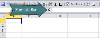
The only time I edit in the cell is when I run a training session because I can zoom in and make the formula larger on the screen.

In practice I only edit in the Formula Bar. When editing in the Formula Bar you can use the Home and End keys to move to either end of the Formula Bar.

FormBar_1

Special Rounding

When you need to round to a certain number, e.g. 5 cents, you can use the MROUND function.

If cell A1 contains a number then the following formula will round the value to the closest 5 cent value.

=MROUND(A1,0.05)

The MROUND function does have some issues – see this blog post.

Formatted table shortcuts

Two of Excel keyboard shortcuts work differently in Formatted Tables (tables that are created using Format As Table icon on the Home ribbon)

Ctrl + Space normally selects the entire column(s). In a formatted table it selects the data in the column. Pressed again it selects the heading and the data pressed once more it selected the whole column.

Shift + Space normally selects the whole row(s), in a formatted table it will select the row within the table.

Excel 2013 – Start screen

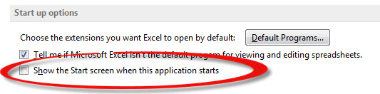
When Excel 2013 opens it display its start window. Many users don’t use templates so it is frustrating. Pressing the Esc key takes you to the familiar grid.

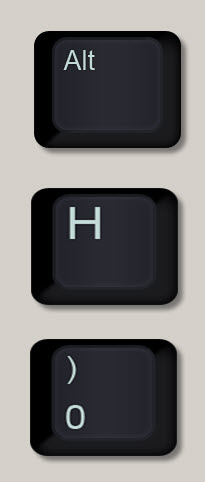
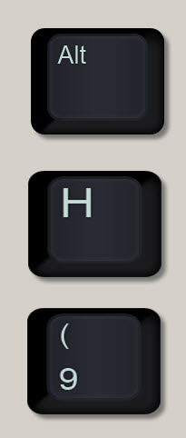
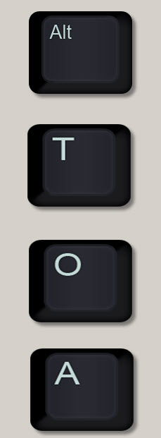
To stop the Start screen displaying use Excel Options. Press in sequence Alt t o (not held down), at the bottom of the dialog untick the Start screen option and click OK.

See image below.

tip_xl2013_01

Formatting part of a cell

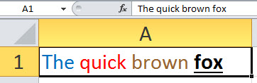
When you are editing a cell you may notice that most of the ribbon icons are greyed out, because you can’t use them. The formatting tools however are not greyed out.

You can select part of the text in a cell and format it differently to the rest of the cell.

See example below.

Tip_Format

Cell Link Shortcuts

If you want to follow a cell link or find cells that are linked to a cell you can use these two keyboard shortcuts.

To follow a link use

Ctrl + [

To find linked cells use

Ctrl + ]

To return after following a link, you can press F5 and then press Enter.

Stop a cell from displaying and printing

You can use a Custom number format to stop a cell or range from displaying and printing.

Select the cell or range

Press Ctrl + 1

Use the 1 on the keyboard not the numeric keypad. In the Number tab click the Custom option (bottom left-hand side)

In the Type box enter

;;;

Click OK

This doesn’t stop the contents of the cell from displaying in the Formula bar.

Counting text in a range

To find out how many cells contain a text string in a range you can use the COUNTIF function and an Excel wildcard character.

To see how many cells contain abc in column A you could use

=COUNTIF(A:A,"*abc*")

This will count abc no matter where it appears in the text eg 123abc, abc123 and 123abc123 will all be counted. It is only counted once per cell.

The * is the wildcard character.

Convert date to its Financial Year End Date

To convert a date to its financial year end date you can use the following formula, assuming the date is in cell A1.

=DATE(YEAR(A1)+(MONTH(A1)>6),6,30)

The (MONTH(A1)>6) part returns TRUE when the month number of the date is above 6. In Excel TRUE = 1, hence 1 is added to the year of the date.

If the month number is 6 or less it returns FALSE and in Excel FALSE = 0, so the year is left unchanged.

A shorter formula that provides the same result is.

=DATE(YEAR(A1+184),6,30)

Displaying Blank or a Zero if an error is encountered

To display a blank cell if an error is encountered use

=IFERROR(A1/B1,"")

To display a zero in a cell if an error is encountered use

=IFERROR(A1/B1,0)

The IFERROR function is available in Excel 2007 onwards.

Adding Positive or Negative Values

To add up the positive values in a column you can use

=SUMIF(A:A,">0")

This will display the total of all the positive values in column A.

To add up the negatives use

=SUMIF(A:A,”<0″)

This will display the total of all the negative values in column A.

Finding how many entries in a column

To find out how many entries there are in a column you can use

=COUNTA(A:A)

This will display how many entries there are in column A.

This is different from the COUNT function which only counts numerical values.

Determine if a Value is Duplicated in a Column

To determine if a value is duplicated in a column you can use

=COUNTIF(A:A,B1)>1

Will display TRUE if the value in cell B1 appears more than once in column A and FALSE if it appears once or not at all.

You can use the above as a logical test in an IF function as well.

Determine if a value is in a range

To determine if a value is in a column you can use the COUNTIF function

=COUNTIF(A:A,B1)>0

Will display TRUE if the value in cell B1 is in column A and FALSE if it isn’t.

You can use the above as a logical test in an IF function as well.

ABS Function

To confirm that two values are within 1 of each other you can use the ABS function.

=ABS(A1-B1)<=1

Will display TRUE if the values in the cells are within one of each other. It will display FALSE if their difference is more than one.

1 is used as it is a common balancing check for rounded numbers.