In Excel it is quite common to test a cell for either a zero or a blank. If either of these two entries are found then you do a particular calculation. There is an easy way to handle this.
Category Archives: Functions
Excel Formula to Extract the Domain
Using the SUBSTITUTE function
I recently read a blog post about using Excel for SEO (Search Engine Optimisation). It mentioned a function to extract a domain from a URL. The function was from Google docs, not Excel. So I wrote an Excel formula to extract the domain from their list of URLs.
Checking Rounded Totals in Excel
Another SUMPRODUCT technique
Rounded values in Excel can pose a few issues. There is a formula you can use that can round a range of values and then SUM the results. This can be used as a check total for rounded values.
SUM or COUNT based on code length in Excel
SUMPRODUCT solution
Let’s say you have codes that have differing numbers of characters and you need to analyse them based on how many characters a code has. There is one function that can SUM and COUNT based on the number of characters in a code.
Another date solution
Formula to the rescue
Getting dates into order is usually a job for Power Query, but not everyone has it or uses it so I still get requests for formulas to fix text dates.
Towards a Simpler IF Function
New function in Excel 2016
Excel 2016 has introduced a new type of IF function to simplify handling multiple conditions. It is called IFS.
Handling DR and CR at the end of numbers in Excel
Sorting out debits and credits
Some systems add DR and CR to the end of numbers when they export into Excel. This renders the values useless for normal calculations. You can use data cleansing techniques to remove the characters using formulas or Power Query. There is one function however that can perform calculations on these types of entries.
How to SUM Text Numbers in Excel
SUMPRODUCT to the rescue
When data is imported into Excel sometimes the values come in as text rather than values. Most functions can’t perform any calculations with text numbers, but one can. See how easy it is to add up text values.
Easier Structures in Excel
Some are easier to use than others
What is the best layout when working with months/quarters/half years and full years? There are a few common structures. I prefer the one that lets you create single formulas that can be quickly copied across and down with as few copies as possible.
Reduce Excel Formula Length
Remove redundant references
When you create formulas that refer to other sheets Excel typically includes the name of the current sheet when you return to the current sheet and refer to a cell.
Some Observations on Structure in Excel
Tables rule
My consulting work recently highlighted a stark contrast in different Excel models and the effort it takes to create or change them. I make some recommendations to make things easier for yourself at the end of this post.
Count Sundays between two dates
SUMPRODUCT shows it flexibility
We’ve all heard the term “A month of Sundays” to describe a long time. Well what if you wanted to count how many Sundays between two dates?
Getting Date Headings Right
Formulas rule
If you are using date-based headings in your reporting models please consider using dates in the headings rather than text. I’ll explain why.
The NETWORKDAYS.INTL Function Has a Unique Trick
Its customisable
The NETWORKDAYS.INTL function was added in Excel 2010. It allows to calculate how may work days between two dates using non-standard weekends. Some countries don’t have Saturday/Sunday weekends.
Making Subtotals Bold
When you use the SUBTOTAL feature in the Data ribbon tab it automatically inserts subtotals in your list – see blog post on it here.
One problem with this is that is only makes the cell with the word Total bold – it doesn’t make the whole row bold.
If you want the whole row to be bold it isn’t hard to fix.
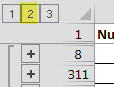
- Select the whole range involved.
- Use the grouping button 2 top left corner. See image below.

- Then hold the Alt key down and press the ; (semicolon key) – this selects just the visible cells.
- Then press Ctrl + b to bold it.
- Click another cell to reset the range and you are done.
How Many Fortnights in a Month
Great for cashflow calculations
I had a question during one of my Date and Times Webinars in February. It was about months and fortnights. I couldn’t answer it during the webinar, but I did follow up with an email with the solution. The answer follows.
SUMIFS Function Warning
Leading zeros are not handled correctly
Most people are unaware that the SUMIFS function has a serious limitation when it comes to codes with leading zeroes. This post shows you how to perform calculations involving codes with leading zeroes. This issue also affects SUMIF, COUNTIF and COUNTIFS.
Converting a Tricky Date Format
I had a question on another post on how to convert Nov 21, 2014 into a date Excel recognises. The solution involves six functions working together.
Creating a Hyperlink in Excel Based on a Search
Teleport to a cell in a data table
Let’s say you have a table of codes and every month there are a few you want to check out. You could use a VLOOKUP to extract all the details for each code, but let’s say you want to view the codes in the table.
Totalling Tip For Excel
Make the most of SUMIF
I wanted to offer a solution to a common problem I see in Excel. It relates to creating totals in data that isn’t structured that well.
Using Lists in Excel
Make the most of Format as Table
It is common to work with lists in Excel. Lists of departments, names and other categories you frequently use. This blog post covers a few techniques that work really well together to create robust reporting systems.
Learning Excel’s Function Arguments
When you start to use a function it can take some time to learn the arguments required and understand what Excel expects for each argument. Eg should it be a cell or a range or either?
When you have the start of a function in the formula bar, you can either press Ctrl + a or click the fx symbol on the left of the formula bar – see image below.
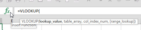
In the image above, the argument in square brackets [range_lookup] is optional. Square brackets around an argument mean it is optional.
This will display a dialog with a listing of the arguments required by a function. The bold names are required, the non-bold names are optional.
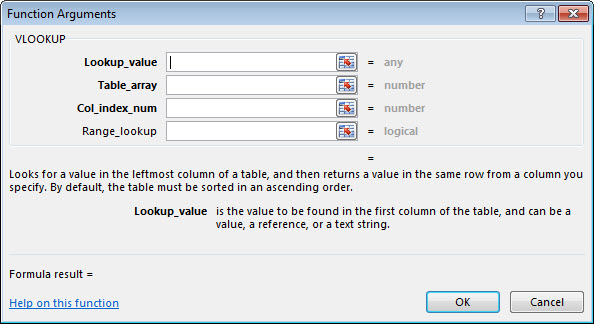
This listing provides a lot more detail on what Excel is expecting for each function argument. This helps you learn more about how to create and use the function.
VLOOKUP and COLUMN Function Warning
Be very careful using these two together
I saw a technique demonstrated recently with VLOOKUP that I hadn’t seen used before and thought at the time, that’s handy. Upon reflection however, I thought that’s a bit dangerous.
The Handy Functions in Excel – LEFT and RIGHT
Simple Defaults
The LEFT and RIGHT functions are great for extracting leading or trailing characters from a text string. Did you know their default setting is handy too?
Summing a range with Errors
If you have a column of values with errors, but you want to see what the values add up to, use the AGGREGATE function (added in Excel 2010).
If column A has the values and errors use
=AGGREGATE(9,6,A:A)
The 9 means SUM. The 6 means ignore errors.
RSM UK
2016-07-06
2016-07-06
Checkerboard Format in Excel
How to get alternate shading in cells
I was looking at a calendar and noticed it used alternately shaded cells, like a checkerboard, for all the dates and thought Excel could do that.
Handling Text and Real Numbers with VLOOKUP
Helping you work with imported data
Sometimes data that comes into Excel with code numbers formatted as text. This can stop VLOOKUP functions from working and return the dreaded #N/A error. With a couple of tweaks you can lookup both real numbers and text numbers in the one formula.
TRANSPOSE Function in Excel
Plus a trick to avoid zeroes displaying
The TRANSPOSE function is one of only a few functions that must be entered as an the array using keyboard entry Ctrl + Shift + Enter (CSE). It allows you to switch a range from going across the sheet, to go down the sheet and vice versa.
Always Refer to Cell A1
If you need to ALWAYS refer to cell A1, regardless of whether row or columns are inserted or deleted, then use the following formula.
=INDIRECT("A1")
This will always display the entry in cell A1 on the current sheet.
Another formula that always refers to cell A1 on the current sheet is
=INDEX(1:1048576,1,1)
Related Posts
“A new financial modelling guide authored by the ICAEW Corporate Finance Faculty and RSM aims to help businesses of all sizes plan and reduce risk. ” – website
If you use or build financial models then this pdf guide may be worth downloading – its free and no email is required – at least when I downloaded it.
Happy reading.
Don’t forget you can read pdfs on your kindle and iPad.