The TRANSPOSE function is one of only a few functions that must be entered as an the array using keyboard entry Ctrl + Shift + Enter (CSE). It allows you to switch a range from going across the sheet, to go down the sheet and vice versa.

Don’t confuse this with the Paste Transpose option in Paste Special. That is simply a copy and paste. It is not dynamic.

Using the TRANSPOSE function creates a link to the range, so that when a value or entry changes, the formula updates.

If there is a blank cell in the target range the TRANSPOSE function will return a zero rather than a blank cell. If you want to show a blank cell see the bottom of this post for a solution.

In the image below we have a report in cells A1:H4.

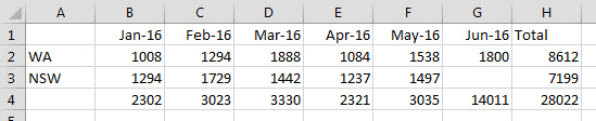
I you want to show that report going down the sheet we can use the TRANSPOSE function to link to the range.

The secret with getting the TRANSPOSE function to work correctly is to select the correct range before creating the formula.

There are a couple of ways to do that.

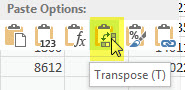
1. Use the Paste Special Transpose option to show you the range you want to create. Simply select the source range and copy it then right clcik the cell you want to start the formula and Clcik the Transpose Option – see image below.Click the yellow fill colour option and this will colour the range you need to select. This makes it easier to select the correct range before creating the TRANSPOSE function.
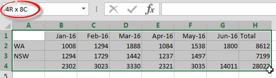
2. Use The Name Box to see how many rows and columns to select. When you use the mouse or keyboard to select a range the Name Box displays the number of rows (R) and columns (C) – see image below.
   In this case the source range is 4 rows high and 8 columns wide. That means we must select a range that is 8 rows high and 4 columns wide before we create our TRANSPOSE function. See image below.

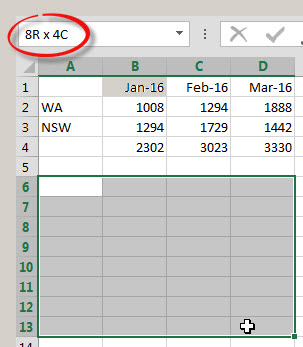
Once you have selected to correct range you then create the formula. In the case above the formula is shown below and must be completed using Ctrl + Shift + Enter.

=TRANSPOSE(A1:H4)

The Ctrl + Shift + Enter entry places curly brackets (braces) around the formula – see image below.

You cannot edit a single cell in an array entered range. You must select the whole range again to edit it.

When you edit the formula the curly brackets will disappear. You must use Ctrl + Shift + Enter after editing as well.

The resulting report is shown below.

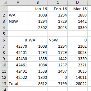
Column A needs to be formatted as a date. As you can see the blank cells in A1 and A4 are shown with zeroes in the linked range in cell A6 and D6.

If you want to avoid displaying zeroes, you can use the following formula that will display a blank for blank cells.

=TRANSPOSE(IF(A1:H4="","",A1:H4))

Remember to use Ctrl + Shift + Enter once you have created the formula.

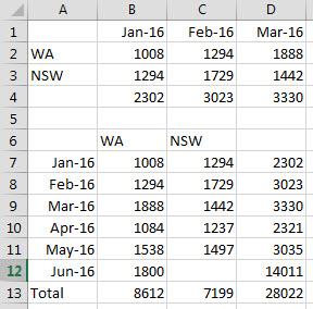
I applied the date format and the above formula – see result below.

Note: When the use Ctrl + Shift + Enter on a range, Excel will not allow you to insert cells, rows or column within that range.