I saw a technique demonstrated recently with VLOOKUP that I hadn’t seen used before and thought at the time, that’s handy. Upon reflection however, I thought that’s a bit dangerous.

The technique involves using the COLUMN function to insert the column reference number for the table in a VLOOKUP. This is the third argument in VLOOKUP and is frequently keyed into the formula, which makes it inflexible to copy. The COLUMN solution, although it seems useful, has a major flaw.

Let’s look at an example. Typically people key in the column number in the VLOOKUP – see yellow highlight in the image below.

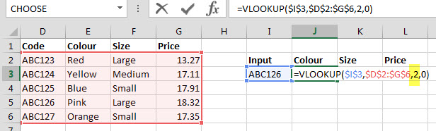
=VLOOKUP($I$3,$D$2:$G$6,2,0)

This means when you copy the formula across you must manually change the 2 to a 3 and the 2 to a 4 for the other two columns. Not an ideal situation.

The solution I saw presented was to use the COLUMN function to provide a sequential number for the column reference in the table as it is copied across.

The COLUMN function returns the column number for the column involved. So =COLUMN(B1) returns 2 and =COLUMN(D1) returns 4.

(By the way I have nothing against using the COLUMN function in general, only how it has been used in this situation.)

The solution is shown in the image below.

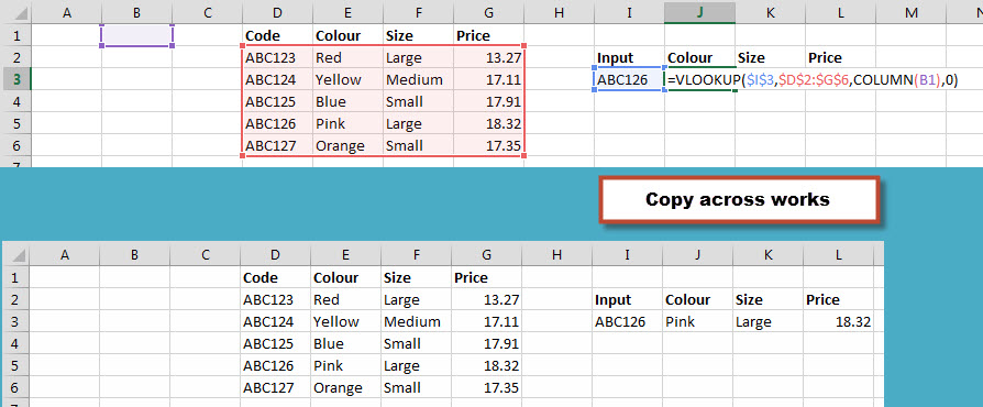
=VLOOKUP($I$3,$D$2:$G$6,COLUMN(B1),0)

So cell B1 is being referred to as it will return the number 2 for the column. This allows you to copy the formula across with no changes.

That seems a great solution, until you realise you are referring to a column outside of the area you are working in and it has no relationship to the calculation you are performing.

This means someone could easily break the formula by inserting a column before column B or deleting column B or column A – see image below.

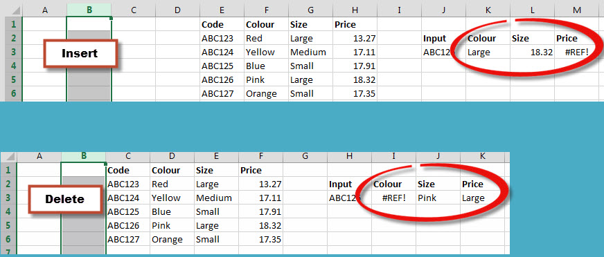
Column B has nothing to do with the calculation, so inserting a column there should be safe, but it breaks the formula.

Locking

For this technique to be safe you have to lock the sheet, which is OK when you have finished the model, but when you are developing the model it is not locked and that is when problems can arise.

Safer Solutions

A simpler solution involves helper cells that hold the column numbers – see example below.

=VLOOKUP($I$3,$D$2:$G$6,J1,0)

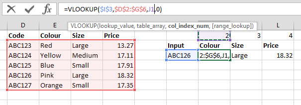
This involves having the column number keyed in to the cells above where you are working. It too has possible problems, but they are less likely to occur as the cells you are working with surround the calculation.

The final way is more complex and involves the MATCH function. See below

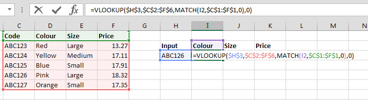
=VLOOKUP($I$3,$D$2:$G$6,MATCH(J2,$D$1:$G$1,0),0)

This is the most robust and preferred solution. It is breakable, but it is much less likely.

Using the COLUMN function could save you some time, but it may also cause you some issues. I would be very careful and protect the sheet if you are using it with VLOOKUP.