It is common to work with lists in Excel. Lists of departments, names and other categories you frequently use. This blog post covers a few techniques that work really well together to create robust reporting systems.

When you work with lists there is a common requirement to always show the list in the same sequence. This makes reading reports more consistent and intuitive.

The easiest way to keep a consistent sequence is to combine the following three techniques:

1. Helper Cells – these are cells that are used to simplify formulas and enable the creation of a single formula that can be copied across and down within a range.
2. INDEX function – this function works extremely well with lists and tables.
3. Format As Table – this feature (on the Home ribbon) is designed to make working with lists and tables a lot easier.

Helper Cells

In our case these will be use to hold sequential numbers that will allow us to maintain the sequence of our list. You can enter these as data entries or use a formula to increment the sequence. I recommend a formula as it simplifies extending reporting ranges.

INDEX Function

The function works very well with vertical ranges (lists) and the syntax is very simple to use.

Syntax

INDEX(Range,Row_Number,Column_Number)

When the range is a single column like a list, you can omit the Column_Number.

For example to refer to cell B4 you could use

=INDEX(B:B,4)

In our case the 4 will be replaced by a cell reference to a Helper Cell and the range will be a table reference.

Format As Table

This feature was an upgrade to an existing Excel feature called Lists in Excel 2003. They renamed it to Format As Table in Excel 2007 and included it on the Home ribbon.

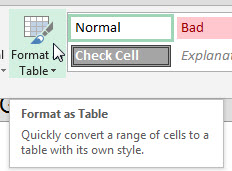
Unfortunately due to its name and Gallery in the drop down, most people think it is a formatting feature.

Its not, its a data feature. To be honest the formatting part is the least of its advantages. This feature tells Excel to treat a table like a little database.

There are lots of advantages to using Format As Table the main one for this example is the fact that the table automatically (automagically??) expands as new items are added to it. This makes it very dynamic and great for reporting systems.

Worked Example

Let’s assume we have 5 states and we always show them in the same sequence in our reports.

I tend to have a dedicated sheet for lists and small tables. A larger table, like a data table, I tend to keep in a separate sheet.

The states list is in a sheet.

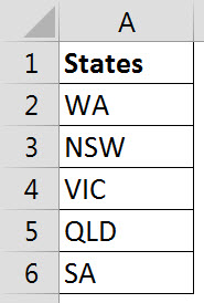
When creating a list, you should always bold the heading row. Excel looks for bold entries to identify header rows.

The golden rule for tables is NO BLANK ROWS!.

If you have blank rows Excel may not automatically identify the full list meaning you have to manually select it. This creates an unnecessary extra step to the process.

Select any cell in the list and press Ctrl + t.

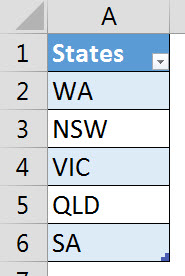
This will apply the default colour of light blue to the list. A dialog opens and the range is confirmed.

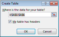
Press Enter to accept the range.

 

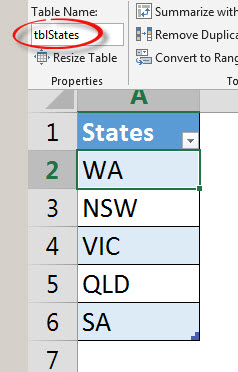
Excel provides a generic Table1 name to your new table. You can modify this and give it a descriptive name in the Design ribbon tab. When you are in the table the Design tab is visible. On the far left of the tab is the name box – see image below. I use a prefix of tbl for my tables. This has a few advantage which I will save for a future blog post.

We are now ready to use the table with the INDEX function.

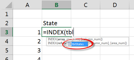
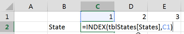
In the image below I start to create the INDEX formula. I type the prefix tbl and the table is shown – pressing the Tab key will input the table name when it highlighted in blue.

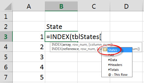
Then I press the [ key which will display the fields (columns) in the table – in this case there is only one column called States.

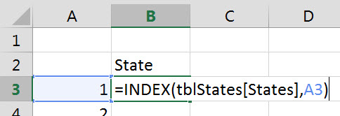
Again I press the Tab key to enter the States field. Then I need a closing ] and type a comma and A3 to link to cell A3 for the row number. The final formula is shown below.

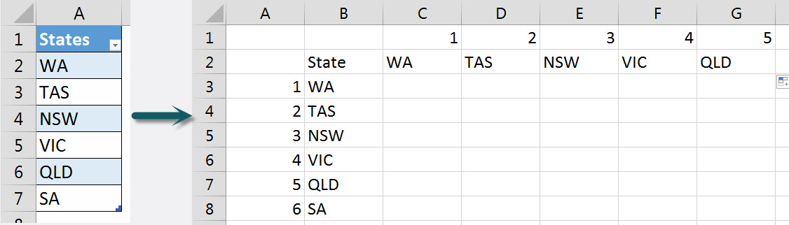
This technique works for creating lists across the sheet as well  – see formula below. See WARNING below.

The technical term for this table reference is a “Structured Reference” but I prefer to call them table references or table names as it is more descriptive.

WARNING:

Be careful using the Fill Handle to copy formulas with table names as the fields can change as you copy across. Use Copy and Paste instead of dragging the Fill Handle. In this case it is OK because there is only on field in the table.

This may look like a long name but as you saw above it didn’t require much typing as Excel was assisting along the way.

Automated List

Now here is beauty of this technique. Let’s say we want to add TAS to our state list.

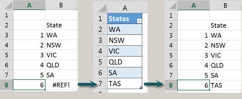
I can copy the formula down and an error will display (see image below). There is no item 6 at the moment, so there is a #REF! error.

As soon as I add TAS to the bottom of my table, the formula will automatically update as shown in the three sections in the image below.

I prefer this INDEX technique, it is more automated than manually entering lists.

Also if you want to adjust the sequence of the list and you use a table, you only need to do it in one place – the table – see below.