If you are using date-based headings in your reporting models please consider using dates in the headings rather than text. I’ll explain why.Examine the image below. The three headings display the same text, but have different entries – the wonders of Excel.

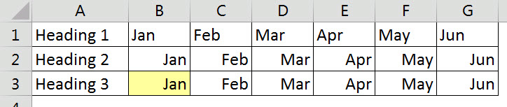The different cell alignment provides a clue to what is in the cells. Text is aligned left in Excel and numbers and dates are aligned right. This is the default – you can over ride the alignment with a format.

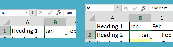
Cell B1 has text in it and cells B2 and B3 contain the same entry, a date – see image below.

Heading 2 ad 3 have a Custom Number format of mmm – see image below. This displays the abbreviated month name.

Heading 2 is preferable over Heading 1 because you can use it to perform date-based calculations using the headings row – eg year to date or quarter date SUMIFS calculations. The text month names are difficult, if not impossible, to use in date-based calculations.

Heading 3 has another advantage over the other two. It is automated.

Cell B3 is yellow because it is an input cell. Cell C3 has a formula that has been copied across to the rest of the cells in the row.

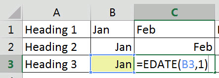
The EDATE function increments dates by months, in the case above, by one month.

So when I change cell B3 to 1/1/18 at the start of the next year, all the dates will update on row 3.

In row 2 you have to change the date and then increment by months for the other cells – a two stage manual process.

Date Tip

Always use the first of the month for your date headings. That makes the dates consistent. The end of the month isn’t consistent and it make calculations that much harder.