Benford’s law is used in auditing to identify data sets that may have been manipulated or adjusted. In my previous post I created a report to analyse a data set based on Benford’s Law. In this post we will create a single formula to create the report and then convert that into a custom function.

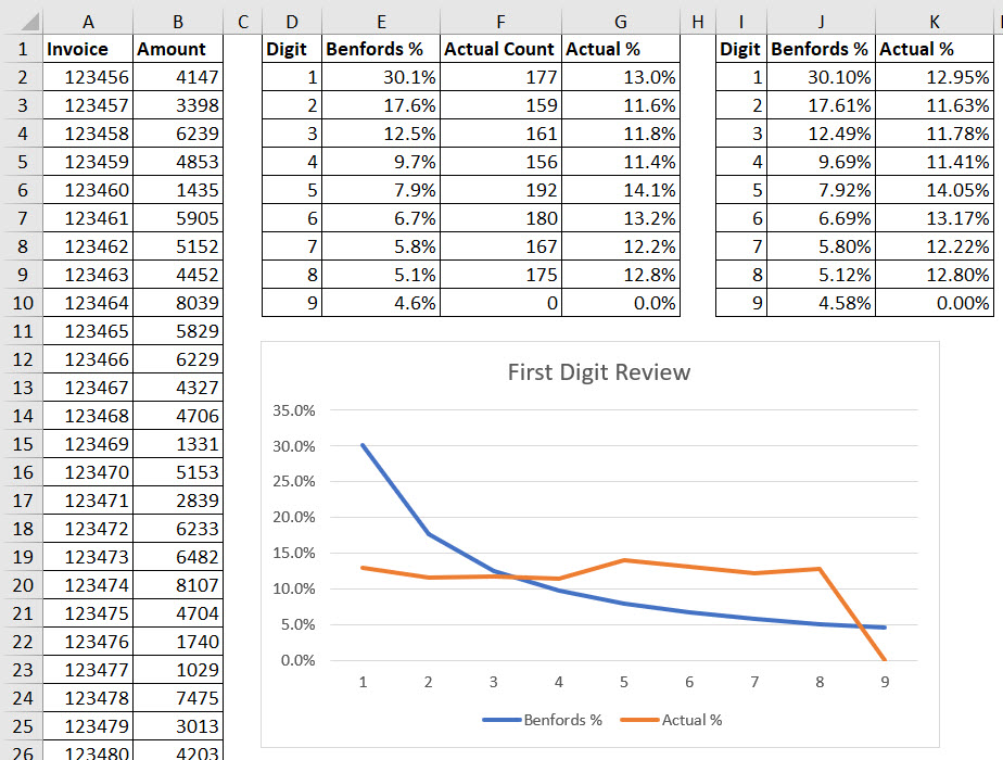
Below is the spreadsheet we reviewed in my last post. You can view the post at the link below.

https://a4accounting.com.au/benfords-law-in-excel-part-one/(opens in a new tab)

You can download the example file using the button at the bottom of this post.

The formulas in the cells are shown in the table below.

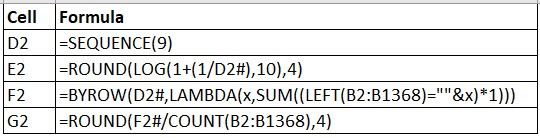
The formulas are also listed below.

=SEQUENCE(9)

=ROUND(LOG(1+(1/D2#),10),4)

=BYROW(D2#,LAMBDA(x,SUM((LEFT(B2:B1368)=""&x)*1)))

=ROUND(F2#/COUNT(B2:B1368),4)

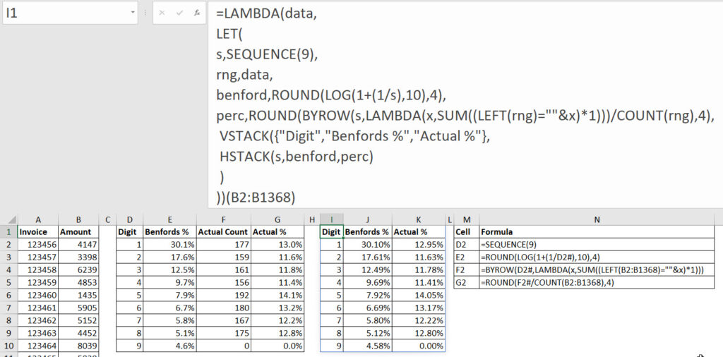
There is a single formula in cell I1 that is creating a report with headings.

The formula is shown in the image below.

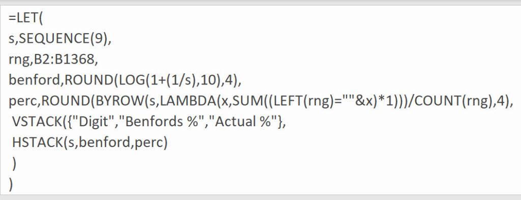
I have split the formula into separate lines in the formula bar using Alt + Enter at the end of each line.

Let’s start at the top and work our way down.

The LET function allows us to use variables in our formula.

The next line defines the variable s as the output of the SEQUENCE function. This captures our sequential numbers from 1 to 9.

The next line defines the variable rng and captures the range that we want to analyse.

The next line defines the variable benford and it uses the formula to calculate the percentages for each of the numbers in the s variable.

The next line defines the perc variable and this calculates the actual percentage based on the rng range.

We now have all the values we need to create the report.

The VSTACK function inserts the headings across the top. It then combines the output of HSTACK function which has created the three column report.

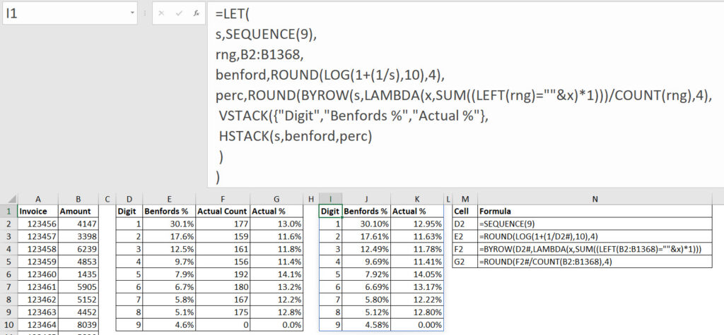
The formula spills down and across to populate the report. The image below shows the formula and the output in cell I1.

Custom function

With such a complex formula it is worthwhile converting it into a custom function that will make it easier to use.

Converting this formula into a custom function is a relatively simple process.

We insert the LAMBDA function at the start and we capture a range which we will call data. We then transfer that data variable into the LET function to define the rng variable and place a closing bracket on the end and we’re done.

The LAMBDA version which we can test with is shown in the image below.

The extra brackets on the end define the range to analyse. That range is passed to the data variable in the LAMBDA function. It is then passed to the rng variable in the LET function.

The final step is to convert the tested LAMBDA function into a custom function.

Copy the whole formula except the extra set of brackets on the end.

Click the Formulas tab.  Click the Define Name icon and paste the formula in the Refers to box at the bottom.

Change the name at the top to fnBENFORD. Click OK.

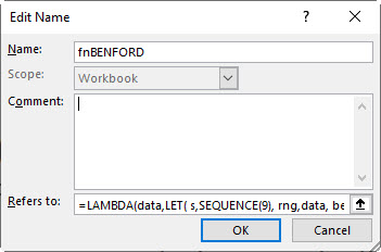
The custom function is ready to use. Note I add fn in lowercase as a prefix for my custom functions to differentiate them from standard Excel functions.

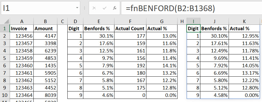
In the image below I have replaced the complex formula with the custom function.

The file with the examples can be downloaded at the button below.