I posted recently about how you can amend a custom list to change the sequence of a slicer – read it here. Here is another tweak I learned from Mr Excel (Bill Jelen).
Tag Archives: data
Let’s TRIM with Dynamic Arrays in Excel
Removing problematic spaces with a single function
Dynamic arrays allow you to use a function normally built to handle a cell, with a range of cells. The TRIM function can remove extra space characters in cells. So with dynamic arrays it can handle ranges.
Find the Closest Value in Excel
Dynamic array solution
On LinkedIn recently someone posted an Excel formula solution lamenting that it was long and complex. That of course was a challenge to me to simplify it.
Excel Custom List Override
In Australia our financial year starts in July. Excel is set up to work with calendar years and we need to do some date gymnastics to have our reports start in July. Here is a hack for Custom Lists that can make some things better in Excel.
Pasting into a Large Formatted Table
There is a quick way to do this
There are times when pasting to the bottom of an existing large, formatted table can take a few minutes to update. There is a quicker way.
When the formatted table is selected there is a Table Design (or Design) tab visible.
On the far left-hand side the Resize Table icon allows you to easily extend the range of the formatted.
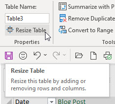
You can amend the range and add sufficient rows to handle the new data in the dialog that opens.
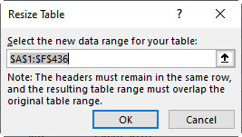
When you paste into an existing formatted table (rather on the end of the table) you will find it will update a lot quicker.
Confirming Names are Unique in Excel
COUNTIFS to the rescue
If you have a list of first names and last names and you want to make sure the list has no duplicates you can use a formula to confirm the names are unique.
Excel Formatted Table Headings
No duplicates allowed
The headings in a formatted table must be unique.
How Many Rows and Columns in a Range
Two functions to the recue
Excel has two functions to answer these questions.
Filter Issue with Excel
Be careful with formatted tables
When you have a filter in place in Excel you typically only affect the visible cells when you edit multiple cells. There is a case when you are affecting all cells not just the visible ones.
Segmenting a Table with Power Query
Slicing and dicing a table
In my previous post I mentioned you should, as far as possible, keep data together in a single table rather than splitting it up between sheets. If you want to split it up for distribution purposes here is an easy way to do it.
Don’t split your data in Excel
If you have Power Query you can consolidate the data
I have received a few questions recently relating to working with data spread across multiple sheets. In general, if the data is in the same layout, keep it in one table.
Excel Drop Down without Data Validation
Alt key solution
Yes, you can create a cell drop down without Data Validation. It uses a built-in technique and is flexible.
One Minute to Excel #3 – Filling in the blanks
No blank looks
Imported data often has missing entries you need to populate.
You can use Power Query, but that duplicates the table.
This technique works on the existing table and is quick and easy to apply once mastered.
Start the clock!
One Minute to Excel #2 – Identify Duplicates
Short, sharp video tips
In the previous video I removed duplicates, in this video we identify duplicates using Conditional Formatting.
I identify the duplicates twice in a minute in this video.
The clock is ticking.
Removing Greyed-Out Slicer Options in Excel
How to tell the Slicer to forget
Sometimes Slicers seem to have a long memory and list entries that are no longer in the current data set. There is a setting to fix this.
Get the Sign Right in Excel
Get the ABS you deserve
I was recently working with some data that had some issues with the sign on the quantities. The quantities should have had the same sign as the associated dollar amount, but they didn’t. Here is how I fixed it.
Excel Slicers Trick
Controlling multiple reports hack
Slicers can control multiple pivot table reports in Excel. The problem is that if you use a slicer on one sheet to filter a report on another sheet it is difficult to see that a filter is in place. This technique also comes with a warning – see bottom of post.
Adding columns to slicers in Excel
Slicers are a great filter interface. Sometimes, due to layout restrictions, you prefer the slicer to go across the sheet rather than down the sheet. Here’s how you do that.
Filter by Cells Value Excel Hack
Excel has a right click Filter option that speeds up filtering by a single value. You can hack that shortcut to do a little bit more.
New XLOOKUP Function in Excel
Part One
It’s finally here, well it is if you have the monthly update cycle of the subscription version of Excel.
Grouping Icon Above Group Rows in Excel
Finding a well hidden setting
The default setting is to have the grouping icon below the grouped rows. But you can switch things and have the icon at the top of the grouped rows.
Creating Groups for Power Queries in Excel
Put some order in your queries
Once you start to use Power Query you may find yourself with quite a few queries in the one file. To make it easier to control them you can use groups to keep similar queries together.
Excel Sort within a Sort
Colour by numbers
Did you know you can sort by colour in Excel? Did you know you can sort ascending or descending within that colour? I was asked a question in a recent webinar and in answering I found out that you can sort within a sort.
Top 5 reports with PivotTable and PivotCharts
Switch the order of the Axis
When you create a top 5 sorted report with a PivotTable, the Pivot Chart isn’t always what you expect, there is an easy solution.
Free Webinar Recording – Introduction to Power Query
Feedback score 94.5% based on 91 responses
In October 2019 I ran my Introduction to Power Query webinar for free (previously it was a paid session). I want to get this information out to as many people as possible. please share this resource with colleagues and your network.
The detailed pdf manual and example file can be downloaded by using the button below. Content listed below the video.
Power Query allows you to automatically perform data cleansing routines on your data sources – no manual intervention required. Simply refresh and your data is ready to use. You can use csv files; txt files; databases and existing Excel tables as your data sources. Learn the basics, plus an advanced technique to automate data cleansing routines on your data sources.
CPD note – if you are claiming CPD for watching this recording you need to keep your own records. People who attend the live sessions receive an annual listing of attendances.
This session covers
- fixing dates so that Excel can recognise them
- formatting columns as text – retaining leading zeroes in CSV files
- deleting unwanted rows and columns from your data
- removing leading and trailing spaces
- populating blank values with zeroes
- populating blanks with entries from above
- correcting trailing minus signs
- unpivot a report – how to convert a report layout into a data table layout
- converting a MYOB report into a data table
Hiding Zero Rows in Excel with No Macros
Filter technique
Over the years I have had regular requests for a technique to hide zero rows in reports. You can use macros but you can also use filters. Let’s see how you can implement a filter solution.
Promoting Headers Issue in Power Query
Be careful if a first row name changes
Promoting headers in Power Query means using the first row as column headers. In Power Query this is a useful and common option. In some cases it is even automated. There is one time though when you don’t want to use it.
Restricting column inputs based on the current month
A data validation solution
Let’s say you have an input range that covers the whole year. You only want users to make entries in the current month column. How can you limit the month entry? The answer is a custom Data Validation.
Power Query Fill Down Doesn’t Work
The fix is easy
Sometimes when working with CSV files in Power Query you may strike the situation where Fill Down doesn’t fill down. Don’t worry there is an easy fix.
Format as Table Extends Data Validation
Another advantage to formatted tables
Excel’s Format as Table feature on the Home ribbon has many advantages. One advantage that isn’t mentioned much is the automatic extension of Data Validations.