Excel has a Remove Duplicates option in the Data ribbon. It keeps the first item and removes any further items that match.

This post was inspired by an idea in one of Mr Excel’s books.

The Remove Duplicates icon is in the Data ribbon.

If you want to see the duplicates that will be removed before you click the above icon, you can use a formula-based conditional format to show you.

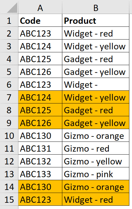
The list we will use is shown below.

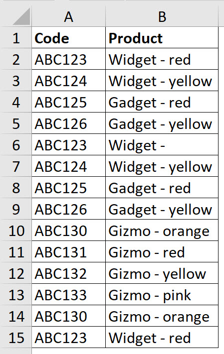
Note: cell B6 is missing a colour, so it shouldn’t be removed even though the code is duplicated.

Excel has a built-in Duplicates conditional format, but it works based on cell entries, not entries across columns. We want to base the conditional format across two columns.

The image below shows the result of the built-in Duplicates conditional format with the default colour.

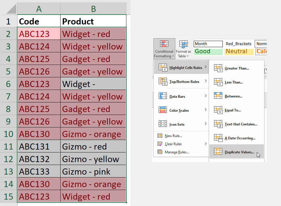
Note that cell A6 is highlighted, but cell B6 isn’t.

Conditional Format

We will use the COUNTIFS function to enable us to identify all but the first entries across the two columns.

1. Select the range A2:B15.
2. On the Home ribbon click the Conditional Formatting icon drop down and choose New Rule, near the bottom of the list.
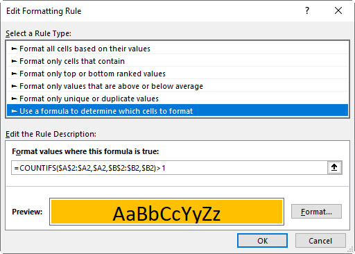
3. Select the last option in the top section “Use a formula to …”.
4. In the Formula box in the bottom section enter the following formula.

   =COUNTIFS($A$2:$A2,$A2,$B$2:$B2,$B2)>1

   

5. Click the Format button and choose a fill colour from the Fill tab – I chose Orange. Click OK.
6. Click OK again to apply the conditional format.

The result is shown below. The highlighted rows will be removed by Remove Duplicates.

How the formula works

When working with a range in a conditional format, the formula you write needs to be built for the first cell in the range involved, in this case the cells in row 2. The formula also needs to return TRUE for the chosen format to be applied.

The ranges used and the $ signs are the important part of this technique. We used a fixed reference for the columns but a relative reference for the rows. This means the range reference will expand down for each row below row 2. You need to use the $ signs on the column references to make sure the correct columns are compared across both columns.

Because we used the >1 comparison the formula will return TRUE for duplicate entries. Remember the range expands as it goes down the sheet. These are the entries that will be removed by Remove Duplicates.

Removing Duplicates

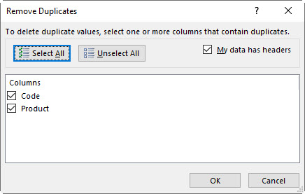
To remove the duplicates, we select a cell in the table and click the Remove Duplicates icon.

In the dialog that opens, make sure both columns are ticked and click OK.

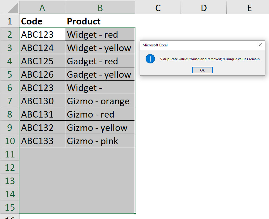
You are told how many duplicates were removed and how many entries remain. Click OK to clear the message box.

You can Undo Remove Duplicates.