An application I use recently updated it’s filtering options to allow you to filter by any filters or all filters. This was a useful addition to the software and I thought that I could apply the same idea to Excel’s FILTER function.

In the image below I have a sales data table in a sheet called data. It is a formatted table and it is named tblSales.

You can download the example file at the button on the bottom of the post.

Added 18 Jul 2023 – you can see a more elegant formula solution than mine in the comments underneath this post. Thanks Rick Rothstein MVP.

In a separate sheet I am filtering the table using the FILTER function – see image below.

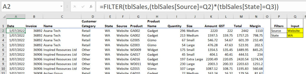
The formula in cell A2 in the above image is shown below.

=FILTER(tblSales,(tblSales[Source]=Q2)*(tblSales[State]=Q3))

This is an example of what is called an AND filter.

The Source column in the table needs to equal Website (cell Q2) AND the State column needs to equal WA (cell Q3). Both filters must be met for the row to display.

An OR filter is shown in the image below. This filter means if the Source column equals Website OR the State column equals WA, then display the row.

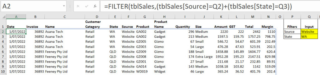
The filter formula for an OR filter is shown below.

=FILTER(tblSales,(tblSales[Source]=Q2)+(tblSales[State]=Q3))

The difference is the use of the + instead of the * between the two conditions.

How the filter criteria works

The way the filter function works is that if the Criteria returns TRUE it displays the row. If the criteria returns FALSE, then it hides the row. The criteria also recognises numbers.

When you multiply two or more conditions together you end up with 0 or 1. 0 is treated as FALSE and 1 is treated as TRUE.

When you add the conditions together in our case with two conditions you can end up with zero, one or two. The zero is still treated as FALSE but the one and the two are treated as TRUE. In fact any numbers other than zero are treated as TRUE. Even negative numbers are treated as TRUE.

LET function

To allow the user to switch between the Any filter and the All filter requires an IF function and we also need to repeat the two conditions. This would make the formula longer. To keep the formula length down we can use the LET function to capture the two conditions in variables.

I’ve added a drop down in cell S2 to allow the user to choose between All and Any filters.

The image below also shows the LET function in cell A2 that is required to make this work.

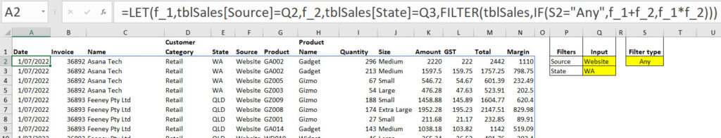
The LET formula in cell A2 is.

=LET(f_1,tblSales[Source]=Q2,f_2,tblSales[State]=Q3,FILTER(tblSales,IF(S2="Any",f_1+f_2,f_1*f_2)))

This uses two variables f_1 and f_2 to capture the first and second criteria. We can then use those variable names in the IF function to choose between the options.

I have defaulted the IF function to use the All filter if cell S2 is blank. The Any filter will only apply if the word Any is in cell S2. The standard filter type is the All filters.

If you need to add more filter criteria, then you just need to add extra variables to capture each criteria and then use those variables within the IF function.