When you create a hyperlink manually in Excel it captures the cell reference. If you insert rows the cell reference in the hyperlink doesn’t update. If you need it to update, this is what you need to do.

Select the cell, let’s say it is B10. Click in the Name Box, this is the box to the left of the Formula Bar.

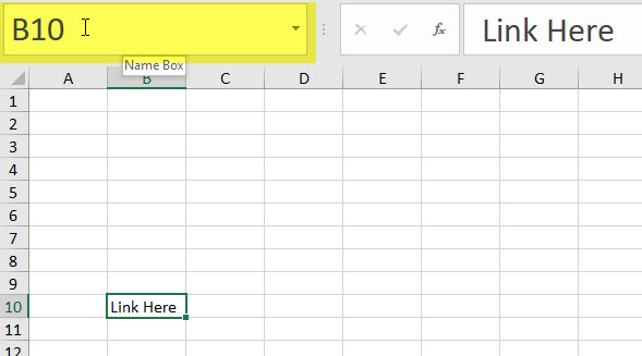
Type LinkCell in the Name Box and press Enter.

The name should stay in the Name Box. This is a range name. You have named cell B10 LinkCell. You can use that name in a formula, and you can use it in a hyperlink.

Don’t insert a space in the name, spaces are not allowed in range names.

Select another cell say D2, press Ctrl + k to open the Insert Hyperlink dialog.

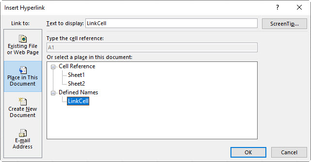
On the left of the dialog, click the Place in This Document button. On the right, select LinkCell in the Defined Names section and click OK. Note: you can change the Text to display at the top of the dialog and you can include spaces.

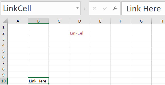
Inserting or deleting rows or columns around the cell will not affect the hyperlink.

If you delete the row or the column that the range name is in, it will break the hyperlink.