Windows File Explorer – New Folder
To insert a new folder in Windows File Explorer use Ctrl + Shift + N.

This page contains resources that I have found useful in my personal and professional life. It contains everything from quotes and books that I like to podcasts and videos.
If you don’t want to scroll through the entire list, you can click on one of the links below to filter the resources by specific category.
I will update this list as I discover new resources. If you have a resource you think I should add, please email me.
To insert a new folder in Windows File Explorer use Ctrl + Shift + N.
To switch to Full Screen mode – great for presentations – use
Ctrl + Shift + F1
Press it again to revert to the normal view.

A quick way to insert a Text Box is by pressing, in sequence (not held down) Alt N X.
A blank Text Box is placed in the middle of the sheet.

To copy an image, graphic or chart simply have the object selected and press Ctrl + D. You can press multiple time to paste multiple times.

If you line the first one up then the others will also line up as you duplicate them.
Do you use Indenting in reports? Example below.
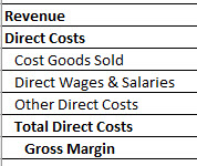
If you do, you make like this keyboard shortcut.
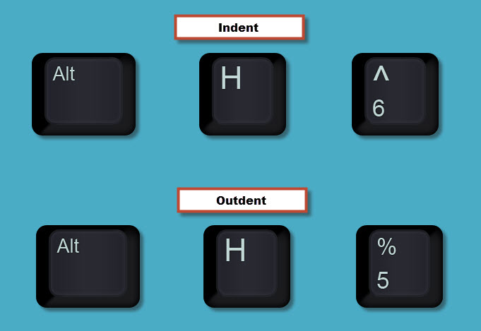
To increase Indenting press Alt H 6 pressed in sequence, not held down.
To decrease Indenting press Alt H 5 (is that an Outdent?)
If you have filters turned on and you are in the heading row of the table you can press Alt + down arrow to open the filter drop down.

You can then use the arrow keys to move up and down.
Apparently this is not widely known, but you should always bold the headings in your tables.
Then when you use Format as Table (Ctrl + t) on the Home ribbon tab the header row will be correctly identified.
This also applies to the Ctrl + Shift + L shortcut to insert the filter drop downs.
It also applies to the ranges used for charts.
In general ALWAYS BOLD your headings – it is something Excel looks for.
Ctrl + b is the bold shortcut.
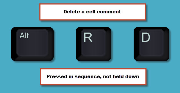
From a question in a recent webinar I found a keyboard shortcut to delete a cell comment.
Alt r d pressed in sequence, not held down.
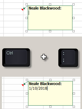
You may know that Ctrl + ; (semi-colon) will insert the current date in a cell.
Did you know it also works in a cell comment?
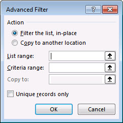
To open the Advanced Filter dialog use Alt A Q pressed in sequence, not held down.

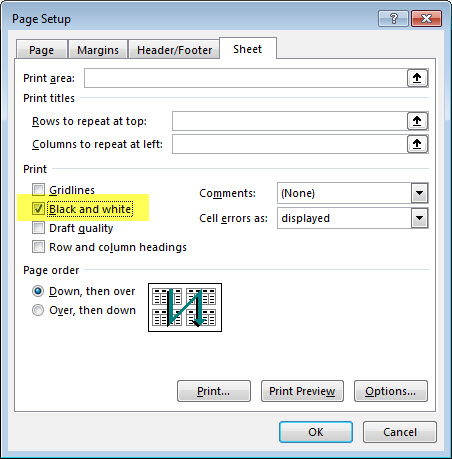
If your sheet has a lot of colour and you want to print it on a black laser printer, one of the Page Setup options can improve the print.
On the Sheet tab of the Page Setup dialog there is a Black And White option – see image below.
This removes all the colour and prints in black only,
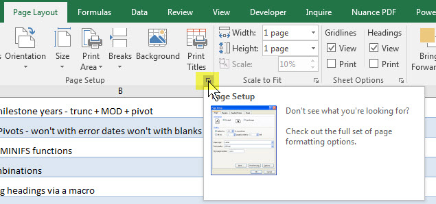
You can access the Page Setup dialog from the Page Layout tab. Click the small arrow on the bottom right of the Page Setup section.
In some large models Excel may calculate for a few seconds after you make an entry.
In most cases you don’t have to wait for Excel to finish calculating before you make your next entry.
Type your entries as fast as you like. Excel will finish calculating once you are done.
Cell comments are useful for instructions and documentation.
If you want to make all the comments on a sheet visible, use Alt v c pressed in sequence, not held down.

Once visible this shortcut also hides all the comments in one go.
This is an old Excel 2003 shortcut that still works.
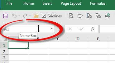
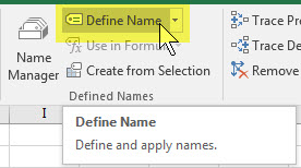
I have found out yet another feature of the Name Box.
The Name Box is on the left of the Formula Bar and above the column letters – see image below.
During a recent macro webinar I tried to create a new range name called Test using the Name Box.
But I also has already created a macro called Test as part of the training.
As soon as I pressed Enter after typing Test into the Name Box to create the Test range name, I was magically transported to the VBA window to the Test macro – Wow!
This means you can’t create a range name in the Name Box that is the same as a macro name.
You have to use the Define name icon on the Formulas tab to do that.
To get the Australian financial year from a date you usually use an IF function based on the month number.
I recently learned a new hack from Matt Allington of Exceleratorbi.
You can add 184 to the date and then use the YEAR function. See table and formulas below.
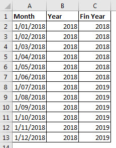
The formula in cell B2 is
=YEAR(A2)
The formula in cell C2 is
=YEAR(A2+184)
Both formulas have been copied down.
A simple solution to a frustrating issue. Thanks Matt.
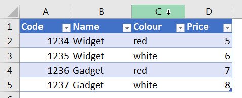
To quickly select a column of data in a formatted table you have a couple of options.
Select a cell in the column and press Ctrl + Space Bar.

This will select the column of data. If you want the heading too, press it again.
You can also select multiple columns before using the shortcut.
This technique can take practice if your headings are in row 1.
If the heading starts in row 2 or below it is easier. See image below.
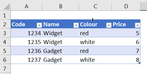
If you point to just above the heading row you will see a downward facing, black arrow. Click this once to select just the data. Click it again to include the heading.
When the heading row is in row 1 you need to do the same but make sure the column letter doesn’t highlight.
The image below is the correct arrow – this will select the column in the table only.
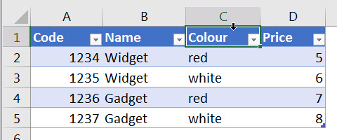
In the image below the arrow shown (because the column letter is highlighted) will select the whole column, not just the data in the table.
When creating long VBA code it is common that the start of an If statement and the matching End If statement may not be visible on the same screen.
When scrolling around trying to understand your code it can be useful to include the If statement itself as a comment following on the same line as the End If command – see examples below.
If x=0 Then 'lots of code If y =1 Then 'lots of code End If 'If y =1 then End If 'If x=0 Then |
The apostrophe is used to specify the start of a comment – you can have a comment following a line of code.
This structure can assist when trying to identify which End If statement relates to which If statement.
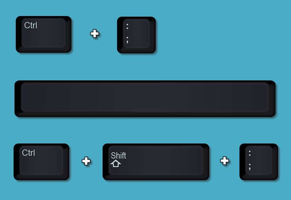
There are shortcuts to enter
There isn’t one to enter both.
You can use them in sequence to achieve a date and a time entry.
In sequence press
Ctrl + ;
Space bar
Ctrl + Shift + :
The space separates the date and time and Excel will recognise the entry as a date and time.
In Excel the “Blanks” option is usually at the bottom of the list. This slows down selecting it.
If you have a lot of entries you need to scroll all the way down to bottom of the list to choose it – see image below.
![]()
But the word “Blanks” is searchable, so if you type b in the Search box – your work is done – no scrolling required – see image below.
![]()
If your column contains text you might need to type in bla.
You learn something new every day.
Today I discovered that you can have columns within a text box.
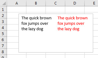
If you right click the text box and choose Format Shape the Task Pane below should open on the right.
Click the third icon (Size and Properties) at the top and then open up the Text Box options.
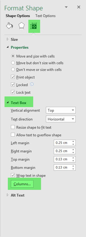
The Columns button allows you to specify how many columns plus the gap between them.
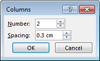
Have fun.
In the structure below let’s assume you want to copy the SUM formula from cell B5 to cell C5.
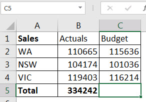
Obviously you could use copy and paste, but that would require a few keyboard presses or mouse clicks.
Given that we already have cell C5 selected we can use
Ctrl + Shift + >

This copies whatever is in the cell on the left to the current cell.
I recently found this keyboard shortcut for MS Word to increase the font size of the selected word(s).

To reduce the font size use

Make your headings bold.
This tip applies to tables and to the structures you use for charts.
Excel looks for the bold format when it reviews tables and layouts to figure out if your table has a headings row.
You can use Ctrl + Shift + L to add or remove the filter icons to a data table. There is also an icon on Data ribbon tab.
This will work more reliably if the headings are bold.
I use the following keyboard combination on the top left corner of the table.
Ctrl + Shift + right arrow (this selects all the headings)
Ctrl + b (this applies bold to the headings)
Ctrl + Shift + L (to turn on filters)
This combination can be done very quickly.
You can just use Ctrl + Shift + L within the table, but sometimes this applies the filter to the wrong row.
A trick to stay in the cell you are editing is to hold the Ctrl key down when you press Enter.

I am amazed how few people know this.
Way back in Office 2007 Microsoft changed the Undo List so that it is NOT cleared whenever you save a file.
You can use Ctrl + z or the Undo icon to undo things you did before you saved the file.
If you close the file that obviously clears the Undo List.
Please let people know this as I find so many people in my training sessions do not know things have changed since Office 2003.
This applies to all MS Office apps.
If you need to clear all the borders from a selected range use
Ctrl + Shift + _ (underline)

Sometimes when running a macro you need to make sure Excel has had time to do something before progressing.
This is typically in large models were it can take time (a few seconds) to do a specific task eg removing a filter or updating an external data source.
You can pause a macro to allow Excel to do something by using the Wait command.
Application.Wait (Now + TimeValue("0:00:02"))
The above code will pause the macro for 2 seconds.
The keyboard shortcut to Refresh All in Excel is

This refreshes all the data connections in the file in one step.
The problem is that on some systems (like mine) this conflicts with an Intel Graphics hot key.
To turn off the graphics hotkeys right click the Desktop and choose Graphics Options, then Hot Keys then Disable. See below.

Big thanks to StackOverflow for covering this issue – link below.
Using Excel’s built-in filtering can speed up your VBA code.
It is important if you are applying filters that you clear any existing filters before you apply a new filter. Otherwise the existing filters will usually affect a new filter you apply.
The line of code below will remove filters on Sheet1 (Sheet1 is the sheet code name that you see on the left side of the VBA screen – it may not be the sheet tab name).
If Sheet1.FilterMode Then Sheet1.ShowAllData
The .FilterMode property is True if a filter is in place on the sheet and False if not.
The .ShowAllData method will return an error if no filter is in place – hence the use of the If statement.
You may know the two keyboard shortcuts below for currency and percentage.

But what you may NOT know is a technique that has been around since the early versions of Excel.
The technique allows you to automatically apply these two formats after you type an entry.
It you type $1000 into a cell and press Enter. Excel will automatically apply the $ format to the cell. The $ sign will not display in the Formula Bar – see below.
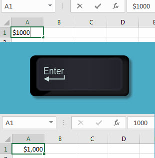
If you type 2.5% into a cell. Excel will automatically apply the standard % format to the cell. The % sign will display in the Formula Bar – see below.

As I mentioned these are really old skills that have been lost over the years since we no longer have Excel manuals – shows my age.