The Format As Table feature has many useful features that are worth taking advantage of. The previous post listed them. The video of this blog is shown at the bottom of the post.

To apply the Format as Table feature to a table you simply select a cell within the table and then, either click the Format as Table icon on the Home ribbon tab, or use the keyboard shortcut Ctrl + t.

The Format as Table icon allows you to choose the colour scheme to apply, the keyboard shortcut uses the default table format. After you click the Format As Table icon you can choose the table format to apply – see image below.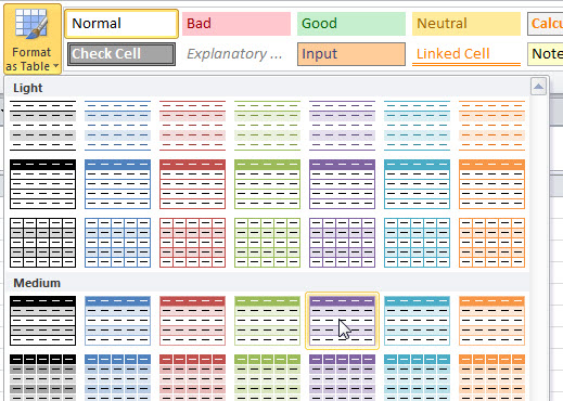

Once you choose the format then you can confirm the table range as shown in the dialog box below. This appears if you use the keyboard shortcut.

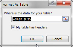
Make sure the “My table has headers” option is ticked and the range is correct. If you do not have blank rows or blank columns in your table then Excel should estimate the range correctly.

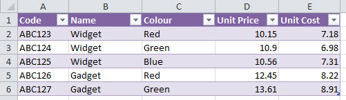
The format will then be applied to the table. Note the filter arrows added to the first row of the table.

If you add another field heading to the right of the table Excel will automatically expand the table to include the new column.

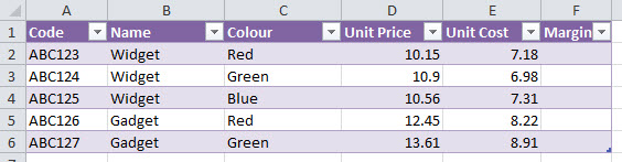
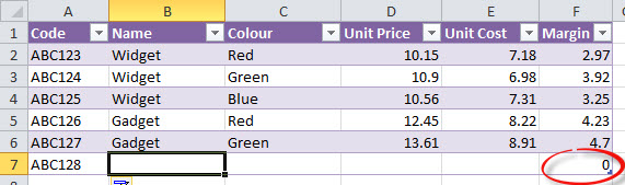
If you create a formula in the new column that refers to other cells in the same row using the mouse or the arrow keys, Excel will automatically insert table names into your formula as shown below.

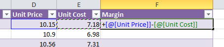
As soon as you press Enter the formula will be copied all the way down the column.

When you have a cell selected within a formatted table a Design ribbon tab is displayed. You can name the table in the Table Name box on the left of the Design ribbon tab.

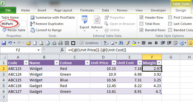
You can also perform calculations outside of the table using the table names. Clicking in the column will insert the table and fields names in the formula. An example is shown in the image below.

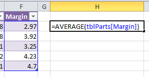
Table names are similar to range names and they automatically expand as data is added to the table.

If you add another record to the bottom of the table Excel will expand the table to include the new record and the formula will also be copied down.

This expanding feature makes a formatted table an ideal data source for a pivot table. When you refresh the pivot table it will automatically include any additional records or fields that have been added to the formatted table.

The video below demonstrates these features.