When you create a checkbox you need to link it to a cell on a sheet to be able to use its result. The user could overwrite that linked cell with a value or text and affect formulas that are using the checkbox linked cell. You can add a validation to make sure the linked cell only contains TRUE or FALSE.

Checkboxes are an easy way to allow the user to turn off or turn on certain calculations or other functionality. But the linked cell can be overwritten and cause issues.

If you want to learn a bit more about using checkboxes check out this post.

There are two ways to stop this happening or at least identify an error.

Inserting a checkbox

To insert a checkbox you need to display the Developer ribbon tab. To do that right click the ribbon and choose Customise the ribbon – then tick the Developer tab.

 

In the Developer tab click the Insert drop down and choose the checkbox icon – top line, third icon.

Then draw a checkbox on the grid. I have drawn it above cell B2 in the image below. You can change the checkbox text but I won’t worry about as I want to focus on the linked cell.

Right click the checkbox and click in the Formula Bar and use the mouse to select cell B2 and press Enter. This links the checkbox to that cell. Click away from the checkbox to deselect it and it is ready to use.

When you tick the checkbox TRUE will display in cell B2 and when you untick the checkbox the word FALSE will display.

Let’s create a simply formula that uses the checkbox linked cell. In cell B4 enter the following formula.

=IF(B2,"ticked","not ticked")

By the way if a cell contains TRUE or FALSE you don’t need to use B2=TRUE you can just use B2 as shown in the formula above.

The Problem

Now here is the problem. The user can enter something else into cell B2, see image below for a couple of examples.

The formula in cell B2 is affected by the entries in B2. Text causes an error but a number is treated like TRUE.

If you tick or untick the checkbox the problem is fixed as TRUE or FALSE will overwrite what is in cell B2.

Data Validation

You can add a Data Validation to cell B2 to stop the user entering something else in the cell.

Select cell B2 and press in sequence Alt A V V this opens the Data Validation dialog. Use the following settings to ensure only a TRUE or a FALSE is entered in cell B2.

The formula used is

=OR(B2=TRUE,B2=FALSE)

If someone tries to enter an invalid entry in cell B2 then the default warning message is displayed.

Validation cell

Unfortunately Data Validation is not a robust solution as someone can paste a value into cell B2 to get around the Data Validation check.

Another option is to use a cell to validate cell B2.

In cell A2 enter the following formula

=OR(B2=TRUE,B2=FALSE)

This is the same formula use in the Data Validation. As long as there is a TRUE or FALSE in cell B2 the validation cell A2 will display TRUE – see below.

If we paste other entries into cell B2 then A2 will display FALSE – see image below.

We can amend our cell B4 formula to first check cell A2 before doing a calculation. The amended formula is

=IF(A2,IF(B2,"ticked","not ticked"),"error")

Blank cell

You may be thinking what if the user deletes the entry in cell B2?

Well a blank cell is treated as FALSE by formulas. See image below where I have deleted the entry in B2.

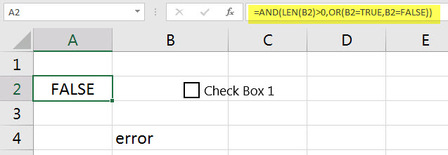
If you wanted to treat a blank cell as an error you could use the following validation formula in cell A2. This will display FALSE if cell B2 is empty or blank.

=AND(LEN(B2)>0,OR(B2=TRUE,B2=FALSE))