Here is a technique that allows you to turn off and turn on the conditional format without actually removing the conditional format. You may want to do this to print a sheet without the conditional formats being applied.
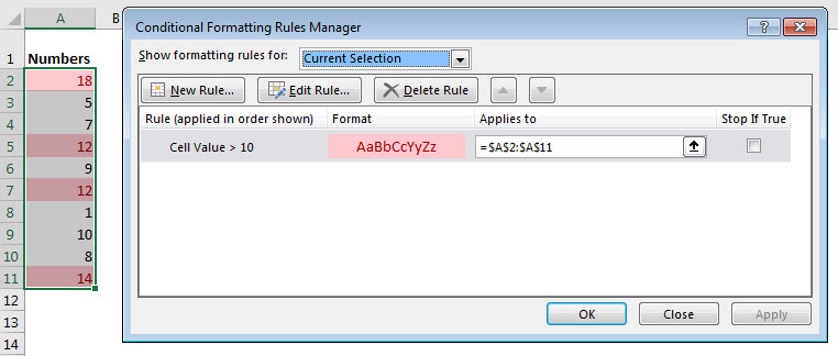
In the image below I have applied a simple conditional format to the range A2 to A11.
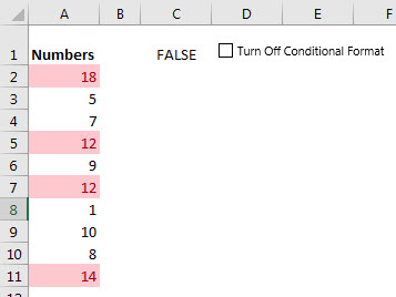
Numbers above 10 are formatted with the light red fill color.
We can amend this conditional format so that it is controlled by a check box.
Check boxes – I have written a detailed blog post on using check boxes here
Check boxes are controls that float above the Excel grid.
When you create a check box you need to link it to a cell on the spreadsheet.
There are a couple of ways to do this.
If you right click the control and then press the Esc key you can click inside the Formula Bar and press the equals sign key and then click on the cell that you want to link to.
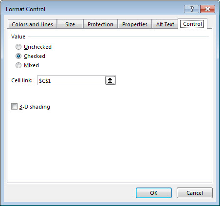
The other way is to right click the control and select Format Control and then click inside the Cell link box and then click the cell that you want to link to.
The checkbox control will display either TRUE or FALSE in the linked cell. A ticked check box will display TRUE, an unticked check box will display FALSE.
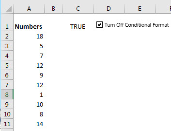
I have added a check box and linked it to cell C1 on the sheet.
We can now amend the conditional format so that it initially looks at the check box result before applying any other conditional formats.
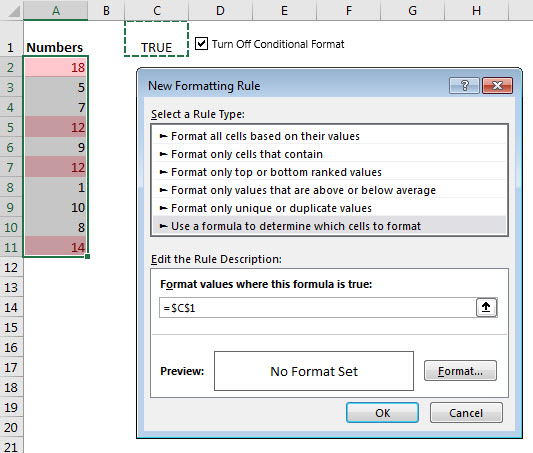
Select the range to work with and then click the Conditional Formatting icon on the Home ribbon and choose New rule and then select the option “Use a formula to determine which cells to format”.
Click inside the formula box and then click the cell C1 which is linked to the check box. Don’t make any other changes just click OK. This will take you back to the Conditional Formatting Rules Manager dialog.
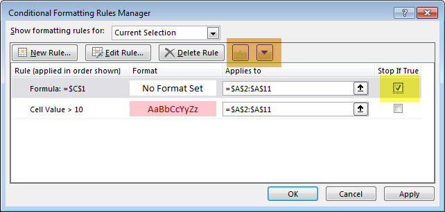
The new rule should be at the top of the list.
On the right-hand side (highlighted in yellow below) there is a check box, tick this. This will stop the remaining conditional formats from being applied if this condition is TRUE.
If you need to move the conditions there are up/down arrows (highlighted in orange in the image above) on the right of the Delete Rule button that allow you to move a selected condition in the Rules Manager dialog.
Ticking the check box will turn off the other conditions, unticking it will apply the conditional format. See images below.

Thank you, I was going crazy trying to do exactly this!
Is there a way to apply the same conditional format to a whole group of checkboxes?
What I mean is, I have a spreadsheet with 40 checkboxes, and I’d like to apply the same conditional format when checkbox is ticked.
Also, I’d love to have a dropdown list if certain boxes are ticked. Is that at all possible?
Thank you again,
A
Sorry, not sure I understand the 40 checkbox question.
In terms of using check boxes to turn off items in a list – that may be possible with the subscription version of Excel which has dynamic arrays.
You can send me an email with an example if you like a4@iinet.net.au.
Hi Nale,
this page is very useful but cane you tell me how I can enable one check box to cancel the other? What I want is that if check box A is checked then checkbox B cannot be checked and vice versa. Have been trying everything without success.
Thank you for your help.
Hi Vanda
You probably need to use two radio buttons as they can only have one selected. Checkboxes are independent. You would need to use a macro to affect the other checkbox.
Regards
Neale
I have the same question as Amaia, but let me explain in more detail.
I have a checklist of items I need to see in the archives, and once I have seen them I tick the checkbox, but this post of yours makes me wonder, can I now work this, so that if A1 = TRUE, turn the text in B1, C1 & D1 to a pale grey and in italics, so that They are partially hidden when glancing at the sheet.
Would I have to create a different conditional format rule for each line on my sheet, or can it be used that if the first cell on any line is TRUE, the following three cells on that line adopt the formatting?
Hi Paul
When you create the Conditional Format (CF) using a formula make sure you use relative references and you can apply the CF to a range in one step.
Regards
Neale