Excel’s built-in finance functions allow you to perform interest and repayment calculations quickly and easily. The PMT function allows you to calculate the monthly repayment on a personal loan or a mortgage.

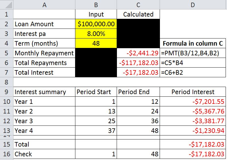
All you need is the principal value, an interest rate and the period of the loan. Excel will do the rest. See rows 1 to 7 in the image below. Yellow cells are for input.

Changing the input cells (B2:B4) changes the repayment. Note the monthly repayment is shown as negative in cell C5.

I received an email question regarding creating a summary table for interest on a loan. I remembered a function I had read about, but never used. I had a play with it and I’m impressed.

CUMIPMT function

There is a function that calculates the cumulative interest between two periods. This function CUMIPMT is perfect for summarising a loan over its life. It makes it easy to create an annual summary table rather than doing a full table with every repayment (That’s what I’d done in the past).

Rows 9 to 16 above have an example summary table which uses the CUMIPMT function and is based on the input cells above.

The syntax of the CUMIPMT function is

=CUMIPMT(Rate, Nper, Pv, Start_period, End_period, Type)

Rate – the interest rate per period

Nper – total number of payment periods for the whole loan

Pv – loan value

Start_period – the starting month number of the loan period to summarise

End_period – the final month number of the loan period to summarise

Type – specifies the timing of the payment.  0 (zero) means payment at end of the period . 1 means payment at the start of the period.

The formula in cell D10 is

=CUMIPMT($B$3/12,$B$4,$B$2,B10,C10,0)

This formula has been copied to cells D11, D12, D13 and D16.

The formula in cell D15 is

=SUM(D10:D13)

Mortgage CUMIPMT Example file.