In the previous post we looked at extracting initials when we only had a first name and a last name in this post, we will look at handling more than two names.

Here is a link to last week’s post that used the new TEXTSPLIT and CONCAT functions to extract the initials.

Extracting Initials in Excel – Part 1

In the image below we can see that our formula from the previous post also works with more than two names.

Instead of all the initials, what if we only wanted to return the first and last initials?

We can use the LET function to help us simplify the formula to extract the first and last initials when there are more than two names.

The LET function allows us to use variables within the formula and that enables us to shorten the formula.

The image below shows the formula that extracts the first and last initials when there are more than two names.

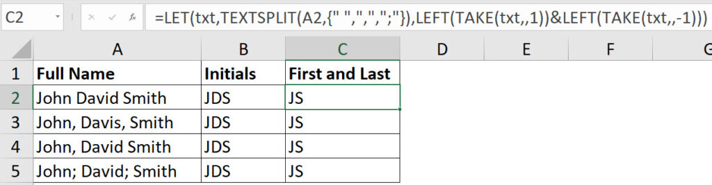
As well as the LET function this formula also uses a new function called TAKE.

The TAKE function allows you to extract from a list based on a number. If you use TAKE with a 1 you extract the first entry. If you use -1 you extract the last entry.

The LET function uses the txt variable to capture the result of the TEXTSPLIT function. With that captured we can then use the TAKE function to extract the first name and the last name from the txt variable. We then use the LEFT function to extract the first character from each name. The & symbol joins the two initials together.

In the image below there is another solution using a single LEFT, TAKE and CONCAT function.

With dynamic arrays there are often many ways to achieve the same result.

This formula is slightly shorter.