If you want to filter by blanks across multiple columns the standard Filter feature can’t help you. You can use the Advanced Filter but that takes time to set up and most users don’t know how to use Advanced Filter.
The solution involves adding a new column to your data to handle your filter requirements.
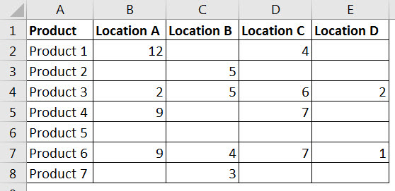
Let’s say we have the following data structure.
We want to identify any location that has a blank in it. If you use the Filter feature it will only display row 6 as Product 5 has a blank in all the 4 locations. We want all the products that have at least one blank.
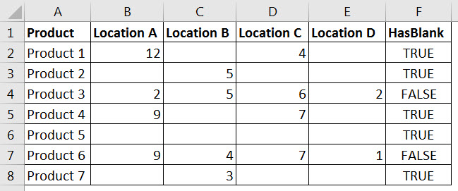
We can add a new column to the data that will allow for this type of filter.
There are many formulas we can use to identify any blank cells in a range. One of easiest to use is in cell F2 in the image above. It is
=COUNT(B2:E2)<4
This counts all the numbers in columns B to E on the same row. If that count is less than 4 it displays TRUE. If there is a number in all four cells it will display FALSE. These types of calculations (displaying either TRUE or FALSE) are called Boolean and are among Excel’s fastest calculations.
We can filter column F by TRUE to see all the rows with a blank in columns B to E. See image below.
If the cells contained text or numbers, you would use
=COUNTA(B2:E2)<4
COUNTA counts all entries. COUNT only counts numeric values (and dates).
If instead of blanks, the list had zeroes you would use
=COUNTIF(B2:E2,0)>0
This counts how many zeroes are in the range and if one or more are found it displays TRUE. If no zeroes are found then FALSE is displayed – see below.
COUNT, COUNTA and COUNTIF can simplify determining when large numbers of cells meet, or are outside, a parameter.


Please note: I reserve the right to delete comments that are offensive or off-topic.