If you have the subscription version of Excel you can create your own functions. One that you may want to create avoids the #DIV/0! error.

In the DAX function language in Power Pivot and Power BI there is a DIVIDE function that avoids divide by zero errors. You can now mimic that function in Excel.

The LAMBDA function and range names allow you to create your own functions that you can use throughout a file.

The typical solution to avoid dividing by zero is to use an IF function as shown in the image below.

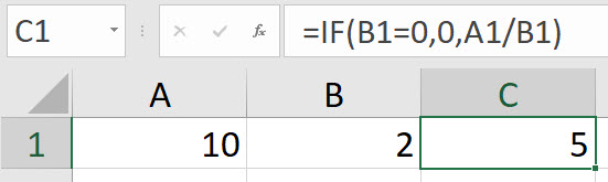
When cell B1 is zero then zero is displayed, otherwise the division is performed.

We want to perform the calculation unless the number we want to divide by is zero. If it is zero, we want to display zero.

LAMBDA function

This new function enables us to set up our function to take inputs and return a value based on calculations we perform.

We need two inputs

• a numerator
• a denominator

But let’s face it most people get confused with those terms. I will use the terms amount and base we want to divide the amount by the base.

When building a LAMBDA we use a special syntax to test it. How you test it is not how you use it. Please hold off any judgement until you have seen the whole process. Below is our example.

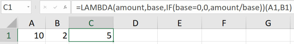
=LAMBDA(amount,base,IF(base=0,0,amount/base))(A1,B1)

The amount and base are variables that we need to populate they will become the arguments of the new function. The (A1,B1) on the end is how we test the function and pass values to the variables. This syntax is unique to LAMBDA.

The amount variable equals the value in A1 and the base variable equals the value in B1. See image below.

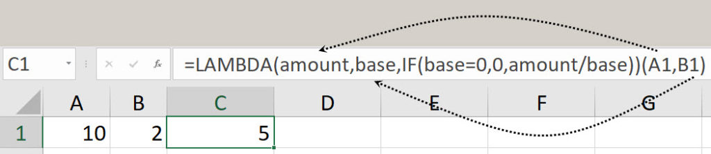
These variable’s values are then used in the IF function within the LAMBDA to perform the test for zero. The LAMBDA function returns the result of the IF function.

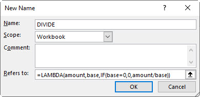
Once tested you can then create your own custom function using a range name. Copy this part of the formula – it leaves off the brackets at the end.

=LAMBDA(amount,base,IF(base=0,0,amount/base))

Click the Formulas tab and click the Define Name icon in the Defined Names section.

In the New Name dialog that opens enter DIVIDE in the Name: box and paste the formula in the Refers to: box and click OK – see image below.

You can now use the new function in cell C1.

=DIVIDE(A1,B1)

See image below.

Function documentation

To make this function easier to use, you can add text to the Comments section of the Name.

In the Formulas tab click the Name Manager icon.

Select DIVIDE and click the Edit button.

In the Comments: box enter text to describe how to use the function and what it does – see image below.

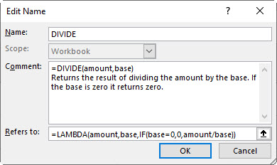
Entry Tip: To enter a line feed in the Comments box use Ctrl + Enter but use the Enter key on the numeric keypad.

Now when you start typing the function name, the description appears – see image below.

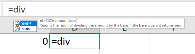
These new custom functions enable you to create shorter and easier to use functions.