The SUBTOTAL function in Excel is quite flexible. The single function allows you to perform 11 different calculations. In this post we will create a custom function to summarise a data set.

This is the third post in a series of posts that will look at how we can automate the SUBTOTAL function to summarise a dataset using a custom function. You can review the two previous posts at the links below.

https://a4accounting.com.au/subtotal-and-dynamic-arrays-in-excel/(opens in a new tab)

https://a4accounting.com.au/subtotal-and-dynamic-arrays-in-excel-part-2/

Currently our problem is that we have a long complex function that provides all 11 functions. We want to simplify it use. A custom function can do that. Our current structure is shown below.

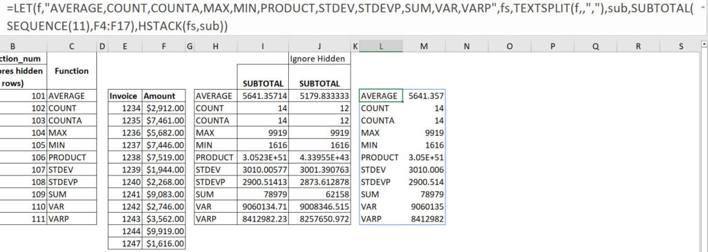
The current formula is in cell L3.

=LET(f,"AVERAGE,COUNT,COUNTA,MAX,MIN,PRODUCT,STDEV,STDEVP,SUM,VAR,VARP",fs,TEXTSPLIT(f,,","),sub,SUBTOTAL(SEQUENCE(11),F4:F17),HSTACK(fs,sub))

This is returning a two column summary of the data set.

LAMBDA function

The LAMBDA function allows us to create custom functions that can simplify complex calculations and make them easier for us and others to use.

This formula is straightforward to convert into a custom function.

To test it we use the LAMBDA in a cell with a special syntax. Once tested we can then create the custom function.

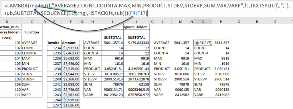
The formula for cell O3 is.

=LAMBDA(rng,LET(f,"AVERAGE,COUNT,COUNTA,MAX,MIN,PRODUCT,STDEV,STDEVP,SUM,VAR,VARP",fs,TEXTSPLIT(f,,","),sub,SUBTOTAL(SEQUENCE(11),rng),HSTACK(fs,sub)))(F4:F14)

This LAMBDA has one argument called rng. This accepts a range from the parentheses on the end of the formula (special syntax). The rng argument is them used in the SUBTOTAL function. See image below.

Custom function

We can now create the custom function using that LAMBDA without the extra parentheses on the end. Copy the LAMBDA function including the = sign.

In the Formulas tab click the Define Name icon.

In the Name box type in fnSUBTOTALL.

In the Refers to box paste in the LAMBDA function – overwrite anything in the Refers to box.

Click OK.

I have entered the custom function in cell R3 – see image below.

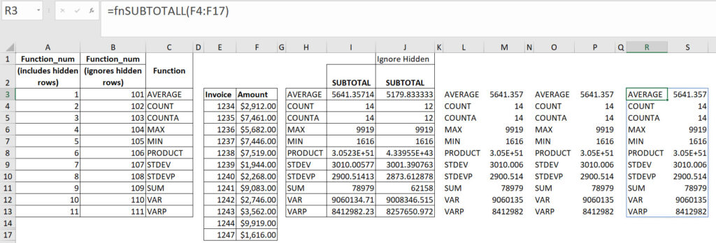
Wow! A summarised report based on a range in a single, short function.

You don’t need the fn prefix on the custom function name. That is something I add to my custom functions to differentiate them from Excel’s standard functions.

In the next and final post, I will provide a few more tweaks to the custom function.