Calculating YTD percentages in Excel isn’t always straightforward, but in some cases you can use Excel’s most flexible function to achieve the result you need.
Let’s have a look at the statistics below.
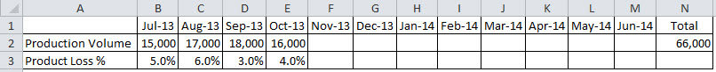
The Loss % cannot be averaged over the period because the volumes vary across the months. We need to do a calculation that takes into account the varying production volumes.
The SUMPRODUCT function can handle this calculation easily.
The SUMPRODUCT function works by multiplying values together and then summing the result. The term PRODUCT in mathematics means to multiply. The product of 2 and 5 is 10. The results of all the multiplications are summed.
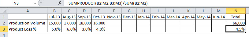
The formula for cell N3 is
=SUMPRODUCT(B2:M2,B3:M3)/SUM(B2:M2)
SUMPRODUCT will multiply B2 by B3, then C2 by C3, then D2 by D3 all the way across the ranges. All the multiplication results are then summed. This will provide the total volume of losses. This is then divided by the SUM of the volumes to provide the ytd loss percentage.
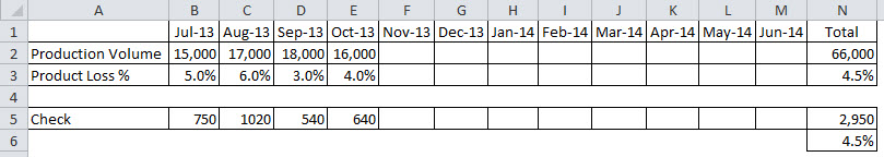
We can check the percentage by manually doing the calculations. See image below.
SUMPRODUCT is an incredibly flexible function and in future blog posts I will expand on its flexibility.
Please note: I reserve the right to delete comments that are offensive or off-topic.