When creating a formula sometimes you need to conditionally choose the column to perform a calculation on. The IF function can be used, but there is a trick to shorten the formula.
This example is based on a request I received recently. We need to do a conditional sum on a conditional column. The example file can be downloaded via the button at the bottom of the post.
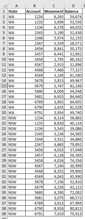
We need to summarise the table below.
The rules are shown in the image below.
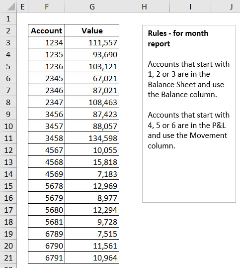
Account numbers starting with 1, 2 or 3 need to use the Balance column (column D). Numbers starting with 4, 5 or 6 need to use the Movement column (column C).
The formula in cell G3 could be
=IF(LEFT(F3)*1<=3,SUMIFS(D:D,B:B,F3),SUMIFS(C:C,B:B,F3))
This uses the IF function to determine which SUMIFS function is required to summarise the account based on the first digit of the number.
The LEFT function when used without a number in its second argument, as above, defaults to the first character. Multiplying by 1 converts the text number returned by LEFT into a real number so it can be compared to 3.
An alternative formula is
=SUMIFS(IF(LEFT(F3)*1<=3,D:D,C:C),B:B,F3)
This shorter formula uses the IF function to return the required range to sum (column D or column C), rather than the whole function. Not everyone knows that the IF function can return a range. This reduces the size of the formula as only one SUMIFS function is required.
Ingenious