The SUBTOTAL function in Excel is quite flexible. The single function allows you to perform 11 different calculations. In this post we will amend the custom function we have created to add an extra column plus headings.

This is the fourth post in a series of posts that will look at how we can automate the SUBTOTAL function to summarise a dataset using a custom function. You can review the three previous posts at the links below.

https://a4accounting.com.au/subtotal-and-dynamic-arrays-in-excel/(opens in a new tab)

https://a4accounting.com.au/subtotal-and-dynamic-arrays-in-excel-part-2/(opens in a new tab)

https://a4accounting.com.au/subtotal-and-dynamic-arrays-in-excel-part-3/

We solved all our problems with a custom function that summarises a dataset in a two-column report. I have tidied up the current structure and it is shown below. You can download the example file at the button on the bottom of this post.

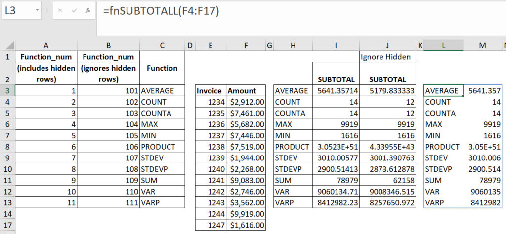
The current formula in cell L3 is.

=fnSUBTOTALL(F4:F17)

This formula spills across and down to create the report with labels.

The LAMBDA function that drives this custom function is.

=LAMBDA(rng,LET(f,"AVERAGE,COUNT,COUNTA,MAX,MIN,PRODUCT,STDEV,STDEVP,SUM,VAR,VARP",fs,TEXTSPLIT(f,,","),sub,SUBTOTAL(SEQUENCE(11),rng),HSTACK(fs,sub)))

Improvements

I thought we could add two improvements.

1. Add another column for the Ignore Hidden Rows results.
2. Add headings to the columns.

These changes are shown and explained below.

Ignore hidden rows

We covered ignoring hidden rows in the first post. SUBTOTAL can ignore the values and entries in hidden rows in it calculations.

To ignore hidden rows we need to add 100 to the SEQUENCE result in the SUBTOTAL results. 1 becomes 101. We can create another variable to hold those results and insert that variable in the HSTACK function to create a third column.

The LAMBDA to test the new column is in cell O3 and is.

=LAMBDA(rng,LET(f,"AVERAGE,COUNT,COUNTA,MAX,MIN,PRODUCT,STDEV,STDEVP,SUM,VAR,VARP",fs,TEXTSPLIT(f,,","),sub_1,SUBTOTAL(SEQUENCE(11),rng),sub_2,SUBTOTAL(SEQUENCE(11)+100,rng),HSTACK(fs,sub_1,sub_2)))(F4:F17)

Remember that the extra parentheses on the end populate the rng variable in the LAMBDA and this allows us to test the LAMBDA formula.

I renamed the sub variable in the LET function to sub_1 and created the sub_2 variable for the ignore hidden rows results. I modified the HSTACK function to include the new variable names. The results can be seen below. I tried using sub1 and sub2 but these weren’t accepted possibly because they are also cell references,

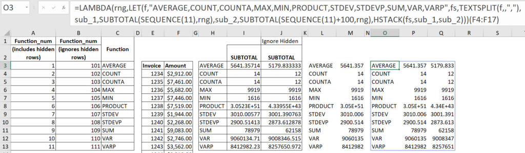
Wow, we now have a three-column report. But then that begs the question, what is the difference between the two result columns? We will need to add column headings to our table.

Adding headings

We have use the HSTACK function, which joins columns together, to create a three column table. There is also a VSTACK function that allows you to add rows to a range. In our case we want to add a heading to the top of each column.

The amended LAMBDA is cell O3 is.

=LAMBDA(rng,LET(f,"AVERAGE,COUNT,COUNTA,MAX,MIN,PRODUCT,STDEV,STDEVP,SUM,VAR,VARP",fs,TEXTSPLIT(f,,","),sub_1,SUBTOTAL(SEQUENCE(11),rng),sub_2,SUBTOTAL(SEQUENCE(11)+100,rng),HSTACK(VSTACK("Function",fs),VSTACK("All Rows",sub_1),VSTACK("Ignore Hidden Rows",sub_2))))(F4:F17)

Each column has a VSTACK to add the heading to it. The image below has the updated LAMBDA.

There is an alternative solution using array syntax. This is more complex, but shorter, as it only requires one VSTACK.

=LAMBDA(rng,LET(f,"AVERAGE,COUNT,COUNTA,MAX,MIN,PRODUCT,STDEV,STDEVP,SUM,VAR,VARP",fs,TEXTSPLIT(f,,","),sub_1,SUBTOTAL(SEQUENCE(11),rng),sub_2,SUBTOTAL(SEQUENCE(11)+100,rng),VSTACK({"Function","All Rows","Ignore Hidden Rows"},HSTACK(fs,sub_1,sub_2))))(F4:F17)

The array syntax {“Function”,”All Rows”,”Ignore Hidden Rows”} creates a heading row across three columns. This heading row is inserted above the whole HSTACK table. Hence only one VSTACK is required.

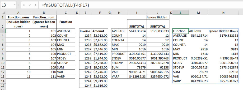
We can now copy one of these new LAMBDAs to the custom function to update fnSUBTOTALL. Remember to omit the extra parentheses on the end.

The final result is shown below. A three-column report with headings.

You can download the example file using the button below.