In last week’s blog post I covered a complex formula to return unique random whole numbers. In this weeks’ post we will look at how we can convert that complex formula into a custom function.

In the image below the formula in cell D2 is.

=TAKE(SORTBY(SEQUENCE(B3,1,B2),RANDARRAY(B3,1,B2,B3)),B4)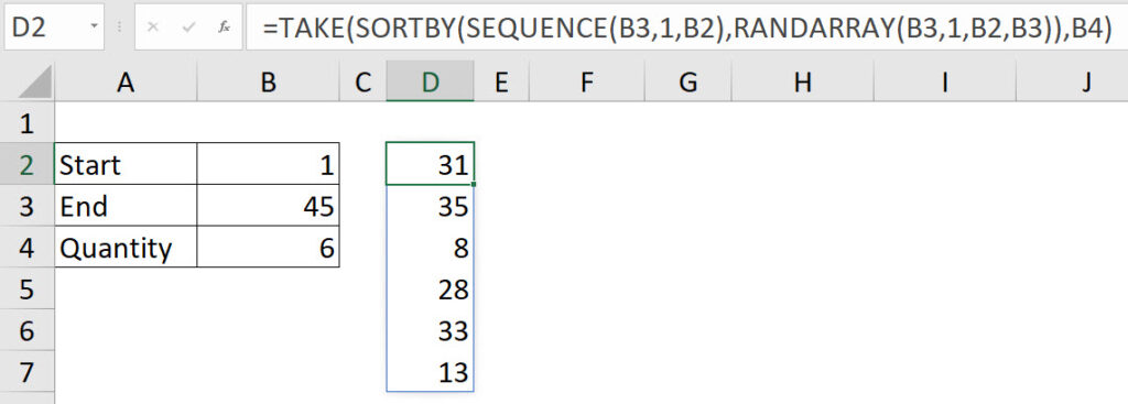

As you can see the formula involves four separate functions. When you have a complex formula that returns a specific result it may be worth creating a custom function to simplify its use.

You can check out the previous post here.

https://a4accounting.com.au/unique-random-whole-numbers-in-excel/

You can download the example file at the button at the bottom of the post.

To create the custom function we need three separate inputs.

1. a high value
2. a low value and
3. how many random numbers to return

The LAMBDA function has a specialised syntax that allows you to test the function before you create the custom function. On the end of the LAMBDA function there is a separate set of parentheses (brackets) that contain the inputs for the LAMBDA function.

Once you have tested the LAMBDA function you can convert it into a custom function by copying it to a range name.

LAMBDA function

The LAMDBA function fo cell D2 is

=LAMBDA(Lo,Hi,Qty,TAKE(SORTBY(SEQUENCE(Hi,1,Lo),RANDARRAY(Hi,1,Lo,Hi)),Qty))(B2,B3,B4)

The LAMBDA has three parameters (variables) Lo, Hi and Qty.

The brackets on the end pass the value in cell B2 to Lo, the value in cell B3 to Hi and the value in cell B4 to Qty.

These values are then passed into the various parameter names within the formula.

Pressing F9 will produce a new set of numbers.

Custom function

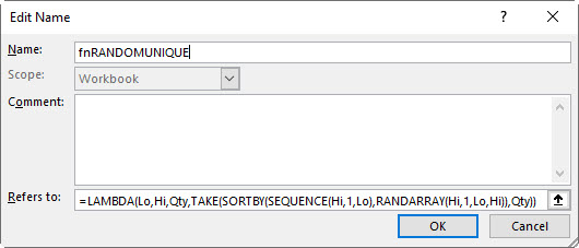
To create the custom function, you copy the LAMBDA function without the extra parentheses on the end and use that in the “Refers to” section of a range name.

Copy the formula

=LAMBDA(Lo,Hi,Qty,TAKE(SORTBY(SEQUENCE(Hi,1,Lo),RANDARRAY(Hi,1,Lo,Hi)),Qty))

In the Formulas tab click the Define Name icon.

In the Name box enter fnRANDOMUNIQUE then click in the Refers to box and paste the copied formula and click OK – see image below.

Note: I use a prefix of fn for all my custom functions. This differentiates the functions from normal Excel functions and allows me to list of all the custom function by typing fn when building formulas.

We can now use the new function in cell D2 – see the image below.

The formula is.

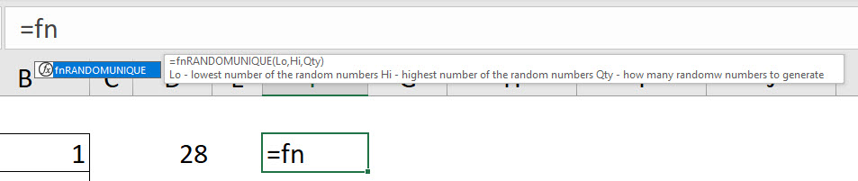
=fnRANDOMUNIQUE(B2,B3,B4)

To make the custom function easier to use you can enter details into the Comments section the Edit Name dialog.

Below is the text entered in the Comments section.

=fnRANDOMUNIQUE(Lo,Hi,Qty)

Lo – lowest number of the random numbers

Hi – highest number of the random numbers

Qty – how many random numbers to generate

Now when you type fn the description is displayed – see image below.

You can download the example file by clicking the button below.