I recently read an Excel VBA book that recommended using numbers instead of VBA constants for message boxes. Please don’t do that. Here’s why.
Excel VBA Mod Operator Problem
Excel has a MOD function that returns the remainder after a division. Excel VBA also has the Mod operator. Unfortunately, they return different results when it comes to negatives.
What matters in life is not what happens to you but what you remember and how you remember it.
Writer and Nobel Prize winner Gabriel García Márquez
Does an Excel range contain sequential numbers?
I have created a custom function to check if a range has sequential numbers. The range doesn’t have to be sorted.
I have long understood that climate change is not only an environmental issue – it is a humanitarian, economic, health, and justice issue as well.
Environmental activist, Frances Beinecke
Excel VBA and the # Symbol
The # symbol is used in Excel sheets for hyperlinks and dynamic arrays. It is also used in VBA for date definitions.
Colour Constants Updated
Thanks to Rick Rothstein MVP for sharing a LinkedIn article he wrote a while back about colour constants. He gave me permission to share the contents in this post. Making your own colour constants.
VBA Color Constants
Simplify using basic colours
In Excel colours are colors. If you want to used basic colours you can use the built-in VBA color constants. This simplifies the code and makes it more descriptive.
Be prepared to appreciate what you meet.
A Fremen proverb from Dune by Frank Herbert.
Extracting Initials in Excel – Part 2
In the previous post we looked at extracting initials when we only had a first name and a last name in this post, we will look at handling more than two names.
Extracting Initials in Excel – Part 1
Extracting initials in Excel can be challenging. That’s because the names can be separated by different characters and there can also be more than two names. Some new functions in Excel can simplify the extraction of initials.
Working with Shapes and Other Graphic Objects in Excel
Shapes can be frustrating to work with in Excel until you find out there are two types of selections with shapes.
Excel, Laptops and Function Keys
Laptop keyboards tend to re-purpose function keys to handle other features. Often the default for the function keys is the laptop features. You then must press the Fn key to access the software function key options. Look out for a FnLock option.
Excel Sheet Names and Emojis
Did you know you can use Emojis on the sheet tabs? The font on sheet tabs is small, so some emojis may not be that effective, but simple emojis can be.
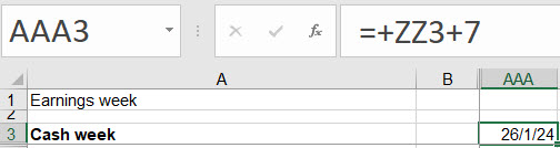
AAA all the way
I started my own weekly cash flow forecast file way back in 2010 and it just ticked over to column AAA!
Excel PivotTable Subtotal Label Trick
I just learned a new trick for labelling subtotal rows in a PivotTable. Hat tip to Ken Puls MVP of Excel Guru for this tip.
Useful Excel Keyboard Shortcuts for Data Entry
When making entries in Excel there are a few keyboard shortcuts worth knowing. These can save you time and effort.
A Better SEARCH Function for Excel
The SEARCH function has a couple of issues that make it difficult to use. This makes it a prime candidate for a custom function to fix its limitations.
Yet Another Post on Hiding Sheets in Excel
If you want to hide sheets and then stop people unhiding them, here is yet another technique.
More Hiding Sheets Macros
These ones work with the selected sheets
It is easy to hide a sheet, you right click the sheet tab and select Hide. Unfortunately, it is just as easy to unhide that sheet once hidden. If you want to hide sheets and make it harder to unhide them, then these macros may help.
More Adjusting in Excel
Following on from last week’s post on a single adjustment formula this post will share a more robust solution for including or excluding adjustments.
Adjusting in Excel
One of the advantages with Excel is that you can usually handle exceptions. In this post I examine a way to handle exceptions or adjustments without using the IF function.
Sparkline Horizontal Axis Technique
Excel Sparkline charts don’t have a horizontal axis. Here is a technique that creates one in the cell above or below the Sparkline. This works best for the Column Sparkline.
In times of change, learners inherit the earth, while the learned find themselves beautifully equipped to deal with a world that no longer exists.
Eric Hoffer
Outside Borders in Excel
How to apply to a range
I use the thin all borders format a lot. But there are times when I need to use the thin outline (outside) borders. This border is not as straight forward to apply to a range.
There is nothing either good or bad, but thinking makes it so.
William Shakespeare, 1564-1616
SUMIFS Wildcard Limitation
SUMIFS can use wildcard characters, but the wildcards only work on text-based codes.
The difficulties of life are meant to make us better, not bitter.
Anonymous
Clearing All Formats in Excel
Sometimes with Excel formatting you just want to clear everything and start again from scratch. You can clear just the formats, and there is an icon you can add to the Quick Access Toolbar to make clearing all the formats earlier.
The greatest value of a picture is when it forces us to notice what we never expected to see.
John W Tukey, Exploratory Data Analysis