Sometimes when you are testing or training in Excel you need to create random entries. That is easy to do with the RANDBETWEEN or RANDARRAY functions. What if you wanted to emphasise some entries more than others in the random list created? There is a way.

Let’s take this simple example.

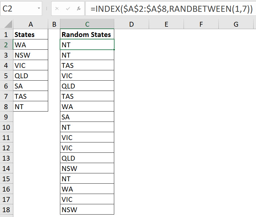
In the image below we have created a random list of Australian States in  column C based on the list in column A. You can download the example file using the button at the bottom of the post.

The formula in cell C2 is

=INDEX($A$2:$A$8,RANDBETWEEN(1,7))

This formula has been copied down to create the random list.

I am from WA. Let’s say I want to have more WA entries than would be randomly generated. How can I achieve that?

The answer isn’t a more complex formula. The answer is put extra WA entries in the list that is used to generate the random entries.

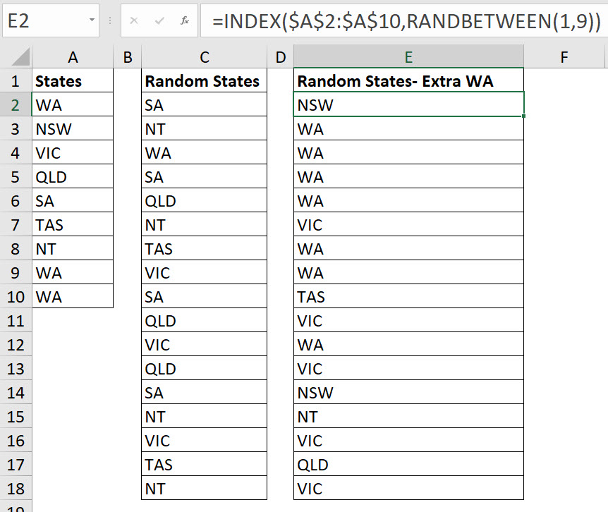
See the image below.

Because WA is in the list three times and the other states are listed once, then WA should be randomly chosen more times. The formula in cell E2 is.

=INDEX($A$2:$A$10,RANDBETWEEN(1,9))

The formula’s structure is the same, we just refer to a longer range A2:A10 and use 9 instead of 7 in the RANDBETWEEN.