With dynamic arrays making array calculations more accessible and easier to use here is a hack for using array syntax in Excel formulas.

What is array syntax?

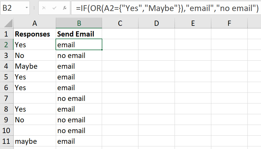
Array syntax allows you to list multiple entries within an Excel formula. As an example have a look at the image below. We have received a response from a survey and we need to email people who has responded Yes or Maybe. If No or a blank then no email is to be sent.

The formula in cell B2 is.

=IF(OR(A2={"Yes";"Maybe"}),"email","no email")

Below is the formula that most people would write.

=IF(OR(A2="Yes",A2="Maybe"),"email","no email")

Because we are looking in the same cell rather than referring to A2 twice we can create a list to check against A2.

That list is created using array syntax.

You start with opening curly brackets (aka braces). You separate the entries of the list with commas or semi-colons and finish with closing curly brackets. Any text needs to be enclosed within quotation marks.

Now if you are creating a longer list typing the array syntax can be problematic. The curley brackets, semi-colons and quotation marks around the text makes typing array syntax time consuming.

Here is a hack to make it easier to create the syntax within the formula. This example is for a short list, but the technique is most useful for a long list.

Type the entries you need in the array syntax in separate cells, one under the other. This is easy to create.

Create the formula and instead of the array syntax refer to the range. See example in the image below.

Edit the formula and use the mouse to highlight the range you have entered. Press the F9 function key. This converts the range into array syntax and press Enter. This keeps the array syntax in the formula – see image below.

Now you can copy the formula down with array syntax.

Using array syntax creates a self-contained formula that can be copied anywhere.

The downside is if you need to edit the entries in the list you need to edit the formula.