Dynamic arrays allow you to use a function normally built to handle a cell, with a range of cells. The TRIM function can remove extra space characters in cells. So with dynamic arrays it can handle ranges.

You will need the subscription version of Excel or Excel 2021 or later version to use this technique.

When you extract data from other systems you can sometimes find that the data has extra spaces in some of the columns. This can affect your use of the data.

Power Query can easily fix this issue, but it requires you to create another data set and to refresh it if things change.

Before Power Query we used to add an extra column with the TRIM function for each row in the table to “fix” the problem column. These days we don’t have to.

If extra spaces are your only problem, then the humble TRIM function can fix a range without the need for an extra column or an extra Power Query data set.

In the table below the state column has both leading and trailing spaces. In practice this is rare. It tends to be either leading or trailing spaces. But for this example I have thrown in both.

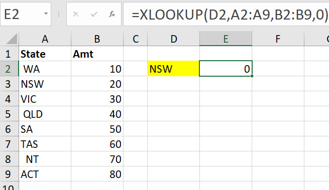
The XLOOKUP function in cell E2 doesn’t work because of the extra spaces in column A.

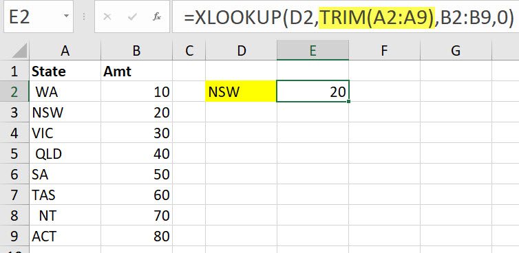
But a simple change to the look up range and it works perfectly. I have highlighted the change in yellow in the Formula Bar in the image below.

The before formula was.

=XLOOKUP(D2,A2:A9,B2:B9,0)

The after formula is.

=XLOOKUP(D2,TRIM(A2:A9),B2:B9,0)

Just wrap the TRIM function around the look up range and the problem is solved.

This technique can also be used for SUMIFS and COUNTIFS plus any other functions that may be affected by leading and trailing spaces.