I wrote a post in 2016 about using INDEX and MATCH to create a hyperlink based on a search result. I thought I would update the technique using XLOOKUP.
You can check out the previous post at the link below.
I will use the same structure as the previous post.
The image below shows the table we want to hyperlink to.
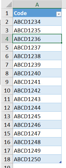
This table is named tblCode.
The images below show the formulas in cells B2 and C2.

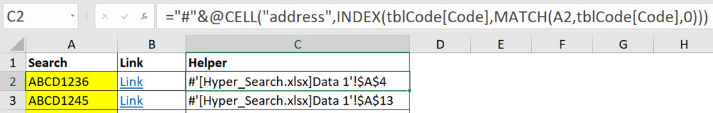
The hard work in done in cell C2. Cells B2 uses the HYPERLINK function and refers to the text string we create in cell C2 and this creates the hyperlink to the cell.
XLOOKUP function
The XLOOKUP function can return a reference to a cell. This means rather than the value in the cell it returns the cell itself. That can be used in the same way as the INDEX-MATCH result. Note VLOOKUP can’t return a reference to a cell.
The new XLOOKUP version of the formula for cell C2 is.
=”#”&CELL(“address”,XLOOKUP(A2,tblCode[Code],tblCode[Code]))
This can be copied down.
It is slightly shorter than the INDEX-MATCH version, but it uses a single function.
It looks up and returns from the same column, tblCode[Code].
The advantage with using the table names (a.k.a structured references) is that as extra data is added to the bottom of the table the range expands to include the extra rows.
The # symbol is used on the front of the reference to identify a bookmark for a hyperlink.
Note the # is now also used as part of dynamic arrays. The # symbol allows you to refer to a spill range. See the post below on it.
Please note: I reserve the right to delete comments that are offensive or off-topic.